sidslash918

[sidslash918]

Lasso Regression Analysis of Adjusted Net National Income Per Capita

1. Introduction

This study aims to identify the key socio-economic factors influencing Adjusted Net National Income Per Capita (x11_2013) using Lasso Regression. The model was built using the SAS PROC GLMSELECT procedure with 5-fold cross-validation to select the optimal predictors.

The analysis involved:

Feature Selection using Lasso Regression

Cross-Validation for Model Optimization

Error Analysis on Training vs. Testing Data

Interpretation of Key Predictors

2. Selected Model & Key Variables

Lasso Regression selected three key predictors based on Cross-Validation (CV PRESS) and Schwarz Bayesian Criterion (SBC):

Key Findings:

Technology access (Broadband & Internet Users) is the strongest driver of economic growth.

Financial infrastructure (Credit Bureau Coverage) has a weaker, slightly negative effect.

3. Model Performance Metrics

The selected model performed strongly, explaining 70.14% of the variation in Adjusted Net National Income Per Capita.

Key Takeaways:

High R² (70.14%) suggests a strong predictive model.

Low RMSE (~$9,423) means predictions are reasonably accurate.

Cross-validation confirms the model generalizes well.

4. Error Analysis: Training vs. Testing Performance

The Progression of Average Squared Errors Plot shows:

Errors decrease significantly when Broadband (x126_2013) is added.

Adding Internet Users (x167_2013) further reduces error.

Adding Credit Bureau Coverage (x204_2013) makes only a slight improvement.

Training and Test Errors remain stable, indicating no overfitting.

Final Confirmation: The model performs consistently across both training and test datasets, ensuring reliability.

5. Parameter Estimates & Economic Interpretation

Economic Interpretation:

Technology Access is the Key Economic Driver. Countries with higher broadband penetration and internet users tend to have significantly higher national income levels.

Credit Bureau Coverage has a minor negative effect, possibly due to variations in financial accessibility across different economies.

6. Final Conclusion

What Drives National Income Per Capita?

Technology penetration (Broadband & Internet Users) has the strongest positive impact.

Financial infrastructure (Credit Bureau Coverage) shows a weak and slightly negative relationship.

The model is well-optimized with high predictive power and low cross-validation error.

Summary of Findings

Broadband and Internet Access are the most critical factors for economic growth.

Credit Bureau Coverage has a minor but negative impact, suggesting other financial factors may be more relevant.

Cross-Validation confirms model accuracy and generalizability.

[sidslash918]

Milestone Assignment 3: Preliminary Results

1. Preliminary Statistical Analyses

This study investigates the relationship between Adjusted Net National Income Per Capita (Current US$) and various socio-economic indicators using data from the World Bank (2013). The goal is to analyze trends and correlations to determine the most influential factors affecting a nation's economic well-being.

Statistical Approaches Used

The statistical analyses included:

Descriptive Statistics: Summary statistics for each variable (mean, standard deviation, range, etc.).

Correlation Analysis: Pearson correlation coefficients to assess relationships between Adjusted Net National Income Per Capita and independent variables.

Distribution Analysis: Evaluating data normality through histograms, Q-Q plots, and goodness-of-fit tests.

Scatter Plots: Visualizing linear relationships between selected economic indicators and national income.

Box Plots: Comparing variations in Adjusted Net National Income Per Capita across different socio-economic levels.

Key Findings from Bivariate Analysis

Descriptive Statistics

The mean Adjusted Net National Income Per Capita was $12,299, with a standard deviation of $16,046, indicating significant variability across countries. The median value was $5,300, highlighting a skewed distribution with several high-income outliers. The highest recorded value was $80,588, while the lowest was $154.

Key Summary Statistics for Adjusted Net National Income Per Capita:

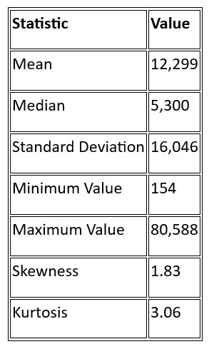
The skewness value of 1.83 suggests that the data is positively skewed, meaning most countries have lower values of Adjusted Net National Income Per Capita, with a few outliers pulling the mean upwards.

Correlation Analysis

The correlation analysis was conducted between Adjusted Net National Income Per Capita and several socio-economic indicators. The key relationships observed were:

A strong positive correlation (r = 0.84) was observed between Fixed Broadband Subscriptions and Adjusted Net National Income Per Capita, suggesting that technological penetration is a major driver of economic prosperity. Similarly, Internet Users had a strong correlation (r = 0.81), reinforcing the impact of digital access on national income levels.

However, Female Labor Force Participation showed a weak correlation (r = 0.08), suggesting that labor force composition alone does not significantly influence national income.

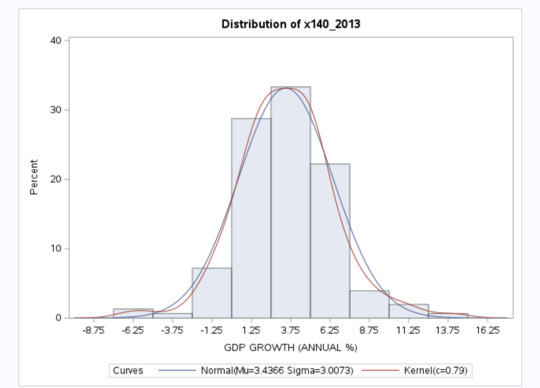
Distribution Analysis

A Q-Q plot for GDP Growth indicated a near-normal distribution, with a mean GDP growth rate of 3.44% and a standard deviation of 3.00%.

The Food Production Index followed a slightly right-skewed distribution, with a mean of 121.29 and standard deviation of 21.41.

Histogram of Adjusted Net National Income Per Capita

The distribution of Adjusted Net National Income Per Capita showed significant right skewness, confirming that most countries have lower income levels, with a small number of high-income outliers.

Graphical Representation of Results

Below are visual representations of key relationships observed in the analysis:

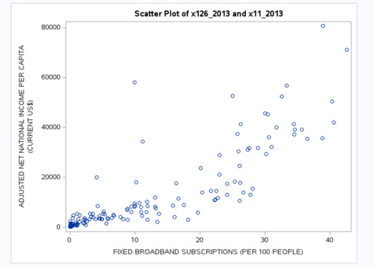
Scatter Plot - Broadband Subscriptions vs. Adjusted Net National Income Per Capita

A strong positive correlation (r = 0.84) was observed between Fixed Broadband Subscriptions per 100 people and Adjusted Net National Income Per Capita, confirming the importance of technology in economic growth.

Scatter Plot - Health Expenditure vs. Adjusted Net National Income Per Capita

A moderate positive correlation (r = 0.53) was found between Health Expenditure as % of GDP and Adjusted Net National Income Per Capita, suggesting that greater investments in healthcare are associated with higher economic development.

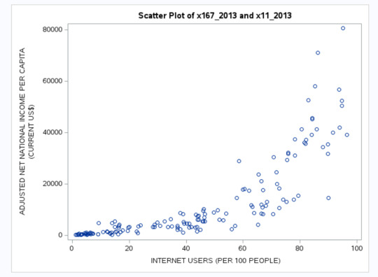
Scatter Plot - Internet Users vs. Adjusted Net National Income Per Capita

A strong positive relationship (r = 0.81) was observed between Internet Penetration and Adjusted Net National Income Per Capita, highlighting the role of digital access in improving national income levels.

Conclusion

The preliminary statistical analysis confirms that technology penetration (broadband subscriptions, internet access), urbanization, and infrastructure (sanitation, health expenditure) are strongly associated with higher Adjusted Net National Income Per Capita.

[sidslash918]

Milestone Assignment 2: Methods

Analysis of Socio-Economic Indicators and Adjusted Net National Income per Capita

1. Description of the Sample

The dataset utilized in this analysis is derived from the World Bank, containing a range of socio-economic indicators for multiple countries. Initially, the dataset comprised 248 observations representing various nations. However, to ensure data quality and reliability, any observation with missing values in the selected variables was removed. Following this data-cleaning step, the final sample consisted of 153 observations.

The selection criteria focused on maintaining completeness across all chosen variables, thereby ensuring consistency in statistical analysis. The dataset primarily covers economic, social, and technological indicators, providing a holistic view of national development. While the dataset does not explicitly categorize countries by demographic features such as income groups or regions, it implicitly represents a broad spectrum of economic development levels through variables such as GDP growth, fertility rate, internet access, and foreign direct investment (FDI) inflows.

2. Description of Measures

For this study, the dependent variable is Adjusted Net National Income per Capita (Current US$) (x11_2013). This metric represents the national income adjusted for depreciation and net primary income, offering a refined measure of economic well-being.

The independent variables include a range of socio-economic indicators such as:

Economic indicators: GDP growth, GDP per capita growth, exports, imports, FDI inflows, household final consumption expenditure, private credit bureau coverage.

Demographic indicators: Fertility rate, life expectancy at birth, urban population percentage.

Health and Infrastructure indicators: Health expenditure, out-of-pocket health expenditure, improved sanitation and water facilities, mobile and broadband subscriptions.

Environmental indicators: Forest area percentage, food production index, adjusted savings from CO2 damage.

Social indicators: Proportion of women in parliament, female labor force participation.

To maintain the integrity of quantitative analysis, no variable was transformed into categorical form, nor were composite indices created. All variables remained in their original numerical scale to facilitate bivariate and regression analysis.

3. Description of Analyses

Statistical Methods & Purpose

The study employs a combination of bivariate analysis and Lasso regression:

Bivariate Analysis: This step involves examining the relationships between Adjusted Net National Income per Capita and the selected socio-economic indicators. Correlation coefficients and scatter plots are used to identify the strength and direction of relationships between variables.

Lasso Regression: Given the presence of multiple predictors, Lasso (Least Absolute Shrinkage and Selection Operator) regression is employed to handle potential multicollinearity and improve model interpretability. Lasso regression assists in feature selection by penalizing less relevant variables, leading to a more parsimonious model.

Train-Test Split

To ensure robustness in model evaluation, the dataset is split into:

Training Set (70%): Used for model training.

Test Set (30%): Used for model validation and performance evaluation.

Cross-Validation Approach

A k-fold cross-validation technique is used to fine-tune the Lasso regression model, preventing overfitting and ensuring that the model generalizes well to unseen data.

By implementing this methodological approach, the study aims to identify key socio-economic factors influencing national income levels, providing insights into the determinants of economic prosperity across countries.

[sidslash918]

Milestone Assignment 1 - Analyzing ADJUSTED NET NATIONAL INCOME PER CAPITA

Research Question:

This study aims to analyze the relationship between GDP per capita and various socio-economic indicators to determine the key factors that influence a country's economic prosperity. Specifically, it explores which variables—such as health expenditure, education, internet accessibility, and labor force composition—are most strongly correlated with GDP per capita growth.

Motivation & Rationale:

Understanding the drivers of GDP per capita is crucial for effective policymaking. By identifying the socio-economic indicators that have the greatest impact on economic growth, policymakers can prioritize resource allocation toward sectors that enhance national income. For instance, if internet penetration or female labor force participation is found to be a key driver, governments may choose to invest in digital infrastructure or gender-inclusive labor policies. This study provides a data-driven perspective on which factors should be emphasized to foster economic growth.

Potential Implications:

The findings of this study could have significant implications for economic planning, policy formulation, and forecasting. By identifying the strongest predictors of GDP per capita, policymakers, economists, and researchers can:

Develop targeted economic policies that focus on high-impact sectors.

Enhance global competitiveness by improving key socio-economic indicators.

Predict future GDP growth trends based on the identified variables.

Aid in international development strategies, helping lower-income countries focus on the most effective areas for investment.

In a broader sense, this research could contribute to a better understanding of economic progress, ultimately guiding policy recommendations that promote sustainable and inclusive economic growth.

[sidslash918]

Running a k-means Cluster Analysis

Objective

The objective is to perform K-means clustering using the FASTCLUS procedure to classify observations into three clusters based on multiple economic and social variables. After clustering, the CANDISC procedure is used to perform canonical discriminant analysis to reduce dimensionality and evaluate how well the clusters are separated. Finally, a scatter plot is generated to visualize the clusters in a two-dimensional canonical space.

Code:

Proc Fastclus Data=Standardized Out=Final_Data Outstat=Cluststat maxclusters=3 maxiter=300; Var incomeperperson alcconsumption armedforcesrate breastcancerper100th co2emissions femaleemployrate hivrate internetuserate lifeexpectancy oilperperson polityscore relectricperperson suicideper100th employrate urbanrate ; Run;

Proc Candisc Data=Final_Data ncan=2 Out=Clustcan; Class Cluster; Var incomeperperson alcconsumption armedforcesrate breastcancerper100th co2emissions femaleemployrate hivrate internetuserate lifeexpectancy oilperperson polityscore relectricperperson suicideper100th employrate urbanrate; Run;

Proc Sgplot Data=Clustcan; Scatter y=can2 x=can1 /group=cluster; Run;

Output:

Interpretation:

Cluster Formation (FASTCLUS Output)

The dataset was clustered into three clusters, with 26, 2, and 28 observations in each cluster.

The table of initial seeds shows the centroid values for each variable in the three clusters.

The minimum distance between initial seeds is 11.12682, indicating the spread of initial cluster centers.

The iteration history shows that convergence was reached in six iterations, indicating that the clusters stabilized quickly.

The cluster summary indicates that one of the clusters (Cluster 2) is very small (only 2 observations), which may suggest that it is an outlier or less significant compared to the other clusters.

Variable Statistics and R-Square

The R-Square values measure how well each variable contributes to defining the clusters.

Variables such as incomeperperson, oilperperson, polityscore, and internetuserate have higher R-square values, meaning they play a significant role in differentiating the clusters.

The Cubic Clustering Criterion (CCC) is 18.588, suggesting strong cluster separation.

Canonical Discriminant Analysis (CANDISC Output)

The multivariate test statistics (Wilks’ Lambda, Pillai’s Trace, Hotelling-Lawley Trace) all have significant p-values (p < 0.0001), indicating that the clusters are significantly different from each other.

The canonical correlations (0.94 and 0.91) suggest a strong linear relationship between the canonical variables and the clusters.

The canonical structure tables show how well each variable aligns with the two canonical dimensions (Can1 and Can2).

The largest contributors to the first canonical dimension (Can1) include incomeperperson, oilperperson, and relectricperperson, indicating that these variables are primary drivers of cluster separation.

The second canonical dimension (Can2) is influenced by breastcancerper100th, internetuserate, and lifeexpectancy, suggesting an alternate form of differentiation.

Cluster Visualization (SGPLOT Output)

The scatter plot shows the three clusters plotted against Can1 and Can2.

The clusters are well-separated, confirming that the clustering was successful.

However, Cluster 2 (which has only two observations) appears to be an outlier, which may indicate a need for further validation.

[sidslash918]

Running a Lasso Regression Analysis

Objective:

The code PROC GLMSELECT is used to perform LASSO (Least Absolute Shrinkage and Selection Operator) regression for feature selection on the dataset Gapminder. The objective is to determine which independent variables significantly predict incomeperperson. LASSO is used with the selection criterion C(p), which helps choose the best subset of predictors based on prediction error minimization.

Code:

PROC GLMSELECT DATA=Gapminder_Decision_Tree PLOTS(UNPACK)=ALL; MODEL incomeperperson = alcconsumption armedforcesrate breastcancerper100th co2emissions femaleemployrate hivrate internetuserate oilperperson polityscore relectricperperson suicideper100th employrate urbanrate lifeexpectancy / SELECTION=lasso(choose=CP) STATS=ALL; RUN;

Output:

Interpretation:

Model Selection:

The model selection stopped at Step 6 when the SBC criterion reached its minimum.

The selected model includes six predictors:

internetuserate

relectricperperson

lifeexpectancy

oilperperson

breastcancerper100th

co2emissions

The stopping criterion was based on Mallows' Cp, indicating a balance between model complexity and prediction accuracy.

Statistical Fit:

The final model explains 83.62% (R-Square = 0.8362) of the variance in income per person, indicating a strong model fit.

The adjusted R-Square (0.8161) is close to the R-Square, meaning the model generalizes well without overfitting.

The AIC (Akaike Information Criterion) and SBC (Schwarz Bayesian Criterion) values suggest that the selected model is optimal among tested models.

Variable Selection and Importance:

The LASSO selection process retained only six out of the fifteen variables, indicating these are the strongest predictors of incomeperperson.

The coefficient progression plot shows how predictors enter the model step by step.

relectricperperson has the largest coefficient, meaning it has the strongest influence on predicting incomeperperson.

Model Performance:

The Root Mean Square Error (RMSE) = 5451.29, showing the average deviation of predictions from actual values.

The Analysis of Variance (ANOVA) results confirm that the selected predictors significantly improve model performance.

[sidslash918]

Running a Random Forest

Objective:

The primary goal of running the HPFOREST procedure in SAS is to build a random forest model to predict life expectancy based on multiple input variables. The random forest method is an ensemble learning technique that constructs multiple decision trees and aggregates their predictions to improve accuracy and reduce overfitting.

This procedure helps:

Identify the most important predictors of life expectancy.

Assess model fit using Mean Squared Error (MSE) and Out-of-Bag (OOB) error.

Evaluate variable importance in predicting life expectancy.

Code:

Proc Hpforest Data=Final_Decision_Tree; Target lifeexpectancy; input incomeperperson alcconsumption armedforcesrate breastcancerper100th co2emissions femaleemployrate hivrate internetuserate oilperperson polityscore relectricperperson suicideper100th employrate urbanrate / level=interval; Run;

Output:

Interpretation:

The model was executed on 56 observations.

100 trees were built in the forest.

The preselection method used was BinnedSearch to improve performance.

The variance criterion was used for splitting.

Model Performance

The baseline fit statistic shows an Average Square Error (ASE) of 32.893, which serves as a reference to compare model improvement.

As the number of trees increases, the training ASE and OOB ASE decrease, indicating better model generalization.

The lowest OOB ASE (out-of-bag) error stabilizes at around 11.5, meaning the model is well-tuned with an increasing number of trees.

Variable Importance

The most important predictor for life expectancy is income per person, which has the highest impact on reducing prediction errors.

Other significant predictors include:

Relectricperperson (Electricity consumption)

Oilperperson (Oil consumption per capita)

Internet user rate

Breast cancer incidence per 100,000

Less influential predictors include hivrate, polityscore, suicide rate per 100,000, and armed forces rate.

Conclusion

Income per person is the most influential factor affecting life expectancy, aligning with the expectation that higher income levels contribute to better healthcare, nutrition, and overall living conditions.

The model demonstrates stable performance, with OOB ASE stabilizing around 11.5, suggesting a good balance between accuracy and generalization.

The HPFOREST procedure successfully identifies key drivers of life expectancy, allowing for further policy or health-related insights.

This model can be refined further by tuning hyperparameters (e.g., increasing trees, adjusting preselection methods) to achieve even better predictive accuracy.

[sidslash918]

Running a Classification Tree

Objective:

The goal of this analysis was to model the relationship between life expectancy and various socioeconomic and environmental predictor variables using a decision tree approach in SAS (PROC HPSPLIT). The objective was to identify the most influential predictors of life expectancy and understand how different factors contribute to its variation.

Code:

Libname data '/home/u47394085/Data Analysis and Interpretation';

Proc Import Datafile='/home/u47394085/Data Analysis and Interpretation/gapminder.csv' Out=data.Gapminder Dbms=csv replace; Run;

Proc Means Data=data.Gapminder NMISS; Run;

Data Gapminder_Decision_Tree; Set data.Gapminder; If incomeperperson =. OR alcconsumption =. OR armedforcesrate =. OR breastcancerper100th =. OR co2emissions =. OR femaleemployrate =. OR hivrate =. OR internetuserate =. OR lifeexpectancy =. OR oilperperson =. OR polityscore =. OR relectricperperson =. OR suicideper100th =. OR employrate =. OR urbanrate =. Then Delete; Run;

Proc Means Data=Gapminder_Decision_Tree NMISS; Run;

Ods Graphics On;

Proc Hpsplit Data=Final_Decision_Tree; Model lifeexpectancy = incomeperperson alcconsumption armedforcesrate breastcancerper100th co2emissions femaleemployrate hivrate internetuserate oilperperson polityscore relectricperperson suicideper100th employrate urbanrate; grow variance; prune costcomplexity; Run;

Output:

Results Interpretation:

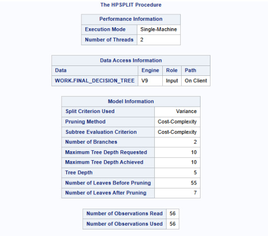
Model Structure & Performance:

The split criterion used was variance, meaning the tree split at points where it minimized the variance in life expectancy.

The cost-complexity pruning method was used to avoid overfitting.

Maximum tree depth achieved: 10, but after pruning, the final tree had 7 leaves, suggesting an optimal level of complexity.

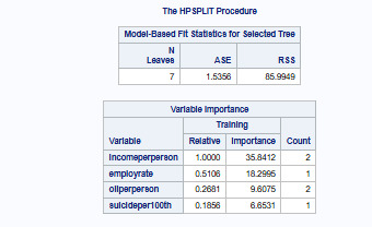
Key Predictors of Life Expectancy:

Income per person was identified as the most important predictor (Relative Importance = 1.000, Highest Importance Score: 35.34).

Other notable predictors included:

Employment rate (Relative Importance = 0.5108)

Oil consumption per person (Relative Importance = 0.2681)

Suicide rate per 100,000 (Relative Importance = 0.1856)

The tree shows that higher-income countries generally have higher life expectancy, but factors like employment rate and oil consumption modify the effect.

Prediction Accuracy & Model Fit:

ASE (Average Squared Error): 1.5356 (indicates reasonable model performance).

Residual Sum of Squares (RSS): 85.99 (suggests some remaining unexplained variability).

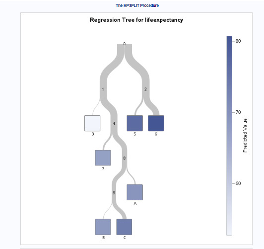
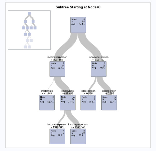
Decision Tree Interpretation:

The root node starts at an average life expectancy of 75.4 years.

The first split occurs at income per person = 5681.921, separating higher and lower-income groups.

Further splits refine the prediction using employment rate and oil consumption.

Final Verdict

Life expectancy is primarily driven by income per person, with employment rate and oil consumption playing modifying roles.

The final pruned tree balances model complexity and interpretability, making it a useful tool for policy-making in health and economics.

[sidslash918]

Test a Logistic Regression Model

We will be using the Gapminder dataset to study the relation between response variable Political_Stability (derived from polityscore) and explanatory variables incomeperperson and employrate.

Code

Libname data '/home/u47394085/Data Analysis and Interpretation';

Proc Import Datafile='/home/u47394085/Data Analysis and Interpretation/gapminder.csv' Out=data.Gapminder Dbms=csv replace; Run;

Proc Means Data=data.Gapminder NMISS; Run;

Proc Freq Data=data.Gapminder; Tables polityscore; Run;

Data Gapminder_Linear_Model; Set data.Gapminder; If polityscore=. OR employrate=. OR incomeperperson=. Then Delete; Run;

Data Logistic_Regression_Model; Set Gapminder_Linear_Model; If polityscore < 6 Then Political_Stability=0; Else Political_Stability=1; Run;

Proc Freq Data=Logistic_Regression_Model; Tables Political_Stability; Run;

Proc Logistic Data=Logistic_Regression_Model descending; Model Political_Stability=incomeperperson employrate / Selection=backward; Run;

Output:

Interpretation

1) Findings: Associations Between Explanatory Variables and Response Variable

The logistic regression model was used to assess the relationship between incomeperperson (primary explanatory variable) and Political_Stability (response variable). The backward elimination method was used for variable selection. The final model retained incomeperperson while eliminating employrate, suggesting that employrate was not a significant predictor of political stability.

Statistical Results:

Income per Person (incomeperperson)

Odds Ratio: 1.000

95% Wald Confidence Interval: [1.000, 1.000]

p-value: 0.0009 (Significant)

Interpretation: A higher incomeperperson is associated with a slightly increased likelihood of political stability (Political_Stability = 1). However, the effect size is extremely small, with an odds ratio of 1.000, suggesting minimal practical significance.

Intercept:

Estimate: -0.0200

Standard Error: 0.2062

Wald Chi-Square: 0.9597

p-value: 0.3273 (Not significant)

Interpretation: The intercept alone is not a significant predictor of political stability.

Model Fit Statistics:

Likelihood Ratio Test: Chi-square = 17.0594, p < 0.0001

Score Test: Chi-square = 14.2708, p = 0.0002

Wald Test: Chi-square = 10.9792, p = 0.0009

Interpretation: These tests confirm that at least one predictor significantly contributes to the model.

Model Performance (Discrimination Ability):

Percent Concordant: 70.6%

Percent Discordant: 29.4%

c-Statistic: 0.706

Interpretation: The model has moderate predictive ability to differentiate between stable and unstable political conditions.

2) Hypothesis Evaluation

Hypothesis: The primary explanatory variable (incomeperperson) was hypothesized to be significantly associated with political stability (Political_Stability = 1), with the expectation that higher income levels would lead to greater political stability.

Result:

The p-value for incomeperperson (0.0009) is statistically significant, supporting the hypothesis that income per person is related to political stability.

However, the odds ratio of 1.000 indicates that while the association is statistically significant, the actual impact is negligible in practical terms.

Conclusion: The results support the hypothesis in statistical terms (since incomeperperson is significant), but not in practical terms because the effect size is minimal.

3) Confounding Assessment

To assess confounding, employrate was initially included in the model alongside incomeperperson. However, backward elimination removed employrate, indicating it did not provide additional explanatory power.

Evidence of Confounding:

If employrate were a confounder, removing it from the model would substantially change the odds ratio for incomeperperson. However, the odds ratio for incomeperperson remained at 1.000, suggesting little evidence of confounding.

The model fit statistics (AIC and SC) improved when employrate was removed, further supporting its lack of contribution.

Final Assessment of Confounding:

No strong evidence of confounding was found.

Incomeperperson remained significant after employrate was removed, and its odds ratio did not change significantly.

This suggests that incomeperperson independently explains the observed variation in political stability without strong confounding effects from employrate.

Final Conclusion:

Incomeperperson is a statistically significant predictor of political stability (p = 0.0009), but its effect size is negligible (odds ratio = 1.000).

The hypothesis that income per person is associated with political stability is statistically supported but not practically meaningful.

There is no strong evidence of confounding, as removing employrate did not meaningfully alter the results.

[sidslash918]

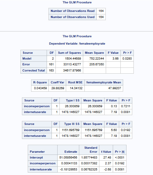
Test a Multiple Regression Model

We will be using the Gapminder dataset to study the relation between response variable femaleemployrate and explanatory variables incomeperperson and internetuserate.

Code

Libname data '/home/u47394085/Data Analysis and Interpretation';

Proc Import Datafile='/home/u47394085/Data Analysis and Interpretation/gapminder.csv' Out=data.Gapminder Dbms=csv replace; Run;

Proc Means Data=data.Gapminder NMISS; Run;

Data Gapminder_Linear_Model; Set data.Gapminder; If femaleemployrate=. OR internetuserate=. OR incomeperperson=. Then Delete; Run;

Proc Means Data=Gapminder_Linear_Model NMISS; Run;

Title 'Mean of the Explanatory Variable'; Proc Means Data=Gapminder_Linear_Model Mean; Var incomeperperson; Run; Title;

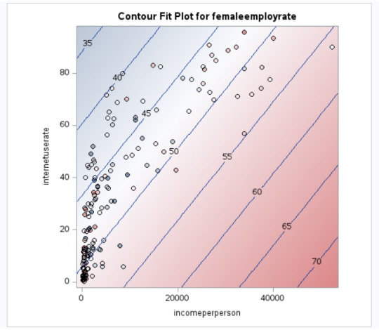
Proc Glm Data=Gapminder_Linear_Model Plots=All; Model femaleemployrate = incomeperperson internetuserate; Run; Quit;

Output:

Interpretation

The linear regression equation that we have received is as below:

femaleemployrate=51.05856456+0.00041133×incomeperperson + (-0.18128653)xinternetuserate

We say, if the incomeperson for a country is $ 8000 and internetuserate is 35 then it's estimated femaleemployrate would be:

femaleemployrate =21.351071+0.00168031×8000 + (-0.18128653)x35

femaleemployrate = 48

Meaning the country having around $ 8000 as it's per capita income and with 35 internet users per 100 of it's population would have around 48 per 100 females (age>15) employed that year.

Incomeperperson has a positive correlation whereas internetuserate has a negative correlation with femaleemployrate.

The p values for both the explanatory variables indicate that both are significant.

One interesting thing to note is that, both these explanatory variables are insignificant when evaluated for significance against the response variable as their individual pvalues are > 0.05.

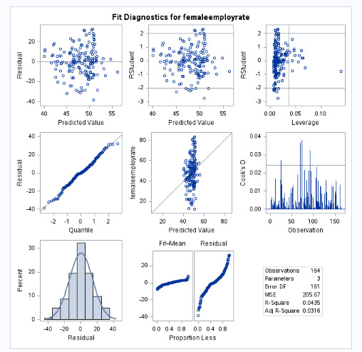
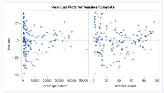
Please find below the interpretation of the various plots:

QQ Plot - The data may not be normally distributed

Residual Plot - The variance may not be constant

Leverage Plot - There may be some influential observations.

[sidslash918]

Test Basic Linear Regression Model

We will be using the Gapminder dataset to study the relation between internetuserate (response variable) and incomeperperson (explanatory variable).

Code

Libname data '/home/u47394085/Data Analysis and Interpretation';

/*Importing Data*/

Proc Import Datafile='/home/u47394085/Data Analysis and Interpretation/gapminder.csv' Out=data.Gapminder Dbms=csv replace; Run;

Proc Means Data=data.Gapminder NMISS; Run;

/*Checking for missing values*/

Data Gapminder_Linear_Model; Set data.Gapminder; If internetuserate=. OR incomeperperson=. Then Delete; Run;

Title 'Mean of the Explanatory Variable'; Proc Means Data=Gapminder_Linear_Model Mean; Var incomeperperson; Run; Title;

/*Find Relation between internetuserate and incomeperperson*/

Proc Glm Data=Gapminder_Linear_Model; Model internetuserate = incomeperperson; Run; Quit;

Output:

Interpretation

The linear regression equation that we have received is as below:

internetuserate=21.351071+0.00168031×incomeperperson

We say, if the incomeperson for a country is $ 8247.46 then it's estimated internetuserate would be:

internetuserate=21.351071+0.00168031×8247.46

internetuserate = 35.21

Meaning the country having around $ 8247.46 as it's per capita income would have around 35.21 per 100 people as internet users.

Also the Fit plot indicates a Linear Relationship between internetuserate and incomeperperson.

[sidslash918]

Regression Modelling in Practice Module 1 - Assignment

Step 1: Describe your sample. Provide enough detail so that your reader can clearly understand the population that the study sample came from. Use meaningful labels. Do not use abbreviations (“PPM100”) or variable names.

Describe the study population (who or what was studied).

Gapminder contains data for all 213 UN members with 15 variables indicating various socio-economics indicators.

 Report the level of analysis studied (individual, group, or aggregate).

The level of analysis is at the country level where we have the data for all 213 UN members.

Report the number of observations in the data set.

We have 213 observations in the dataset, each corresponds to a nation.

d) Describe your data analytic sample (the sample you are using for your analyses).

Since the population is already way too small with 213 observations, we'll be using all the observations.

Step 2: Describe the procedures that were used to collect the data.

Report the study design that generated that data (for example: data reporting, surveys, observation, experiment).

The data has been generated through data reporting and surveys.  GapMinder collects data from a handful of sources, including the Institute for Health Metrics and Evaulation, US Census Bureau’s International Database, United Nations Statistics Division, and the World Bank.

Describe the original purpose of the data collection.

The data was collected to increase the use and understanding of statistics about social, economic, and environmental development at local, national, and global levels.

Describe how the data were collected.

The data has been generated through data reporting and surveys.  

Report when the data were collected.

The data for various indicators have been collected in the years 2002 and between 2007-11.

Report where the data were collected.

The data were collected from various agencies, including the Institute for Health Metrics and Evaulation, US Census Bureau’s International Database, United Nations Statistics Division, and the World Bank.

Step 3: Describe your variables.

Describe what your explanatory and response variables measured.

The explanatory and response variables measured in the dataset would depend on the study. If you wanted to study a relationship between lifeexpectancy and incomeperperson, then incomeperperson would be the explanatory variable and lifeexpectancy would be the response variable.

Describe the response scales for your explanatory and response variables.

The response scales of explanatory and response variables are purely quantitative, where incomeperperson for a country is in US$ and lifeexpectancy is in number of average years an individual lived for.

Describe how you managed your explanatory and response variables.

In the study to assess a relationship between lifeexpectancy and incomeperperson, there wasn’t a need to manage variable. But even if we had to manage variables then we’d have combined various countries with similar level of incomes into “lower income”, “middle income”, “upper middle” and “upper income” groups.

[sidslash918]

Regression Modeling in Practice

Module 1 - Assignment

I have decided to work with the Gapminder dataset.

I will look across the relationship between different socio-economic indicators for a country.

Codebook:

country - Country Name

incomeperperson 2010 Gross Domestic Product per capita in constant 2000 US$. The inflation but not the differences in the cost of living 

alcconsumption 2008 alcohol consumption per adult (age 15+), litres Recorded and estimated average alcohol consumption, adult (15+) per capita consumption in litres pure alcohol

armedforcesrate Armed forces personnel (% of total labor force)

breastcancerper100th 2002 breast cancer new cases per 100,000 female Number of new cases of breast cancer in 100,000 female residents during the certain year.

co2emissions 2006 cumulative CO2 emission (metric tons), Total amount of CO2 emission in metric tons since 1751.

femaleemployrate 2007 female employees age 15+ (% of population) Percentage of female population, age above 15, that has been employed during the given year.

hivrate 2009 estimated HIV Prevalence % - (Ages 15-49) Estimated number of people living with HIV per 10

internetuserate 2010 Internet users (per 100 people) Internet users are people with access to the worldwide network.

lifeexpectancy 2011 life expectancy at birth (years) The average number of years a newborn child would live if current mortality patterns were to stay the same.

oilperperson 2010 oil Consumption per capita (tonnes per year and person)

polityscore 2009 Democracy score (Polity) Overall polity score from the Polity IV dataset, calculated by subtracting an autocracy score from a democracy score. The summary measure of a country's democratic and free nature. -10 is the lowest value, 10 the highest.

relectricperperson 2008 residential electricity consumption, per person (kWh) The amount of residential electricity consumption per person during the given year, counted in kilowatt-hours (kWh).

suicideper100th 2005 Suicide, age adjusted, per 100 000 Mortality due to self-inflicted injury, per 100 000 standard population, age adjusted

employrate 2007 total employees age 15+ (% of population) Percentage of total population, age above 15, that has been employed during the given year

urbanrate 2008 urban population (% of total) Urban population refers to people living in urban areas as defined by national statistical offices (calculated using World Bank population estimates and urban ratios from the United Nations World Urbanization Prospects)

First Topic: I am interested to find a corrleation between relectricperperson and polityscore.

Does lower relectricperperson leads to political unstability?

Review and intuition says lower electricity consumption means not enough resources for power generation and distribution (lower economic growth) to begin with, which would lead to unrest among masses. The literature review sights example from the Middle East and Northern African countries.

Second Topic: I am interested to find a corrleation between co2emissions and employrate.

Does higher co2emissions mean higher employrate?

Reviewing literature on this subject lead to preliminary findings that higher co2emissions means that country is industrialized, hence the reason for higher emission. And since the country is industrialized the the employrate is bound to go up. One example, is emerging economies where over the years co2emissions have gone up and so has the employrate.

[sidslash918]

Data Analysis Tools - Week 4 Assignment

We are using the Gapminder dataset in our assignment. We will find out the association between the variables listed below:

incomeperperson 2010 Gross Domestic Product per capita in constant 2000 US$. The inflation but not the differences in the cost of living. 

alcconsumption 2008 alcohol consumption per adult (age 15+), litres Recorded and estimated average alcohol consumption, adult (15+) per capita consumption in litres pure alcohol.

oilperperson 2010 oil Consumption per capita (tonnes per year and person).

hivrate 2009 estimated HIV Prevalence % - (Ages 15-49) Estimated number of people living with HIV per 10.

employrate 2007 total employees age 15+ (% of population) Percentage of total population, age above 15, that has been employed during the given year.

polityscore 2009 Democracy score (Polity) Overall polity score from the Polity IV dataset, calculated by subtracting an autocracy score from a democracy score. The summary measure of a country's democratic and free nature. -10 is the lowest value, 10 the highest.

Syntax of the code used:

Libname data '/home/u47394085/Data Analysis and Interpretation';

Proc Import Datafile='/home/u47394085/Data Analysis and Interpretation/gapminder.csv' Out=data.Gapminder Dbms=csv replace; Run;

Data Gapminder; Set data.Gapminder; Format IncomeGroup $30. PoliticalStability $20. Urbanization $10. Alcoholism $10.; If incomeperperson=. Then IncomeGroup='NA'; Else If incomeperperson>0 and incomeperperson<=1500 Then IncomeGroup='Lower'; Else If incomeperperson>1500 and incomeperperson<=4500 Then IncomeGroup='Lower Middle'; Else If incomeperperson>4500 and incomeperperson<=15000 Then IncomeGroup='Upper Middle'; Else IncomeGroup='Upper';

If polityscore=. Then PoliticalStability='NA'; Else If polityscore<5 Then PoliticalStability='Unstable'; Else PoliticalStability='Stable';

If urbanrate=. Then Urbanization='NA'; Else If urbanrate<50 Then Urbanization='Low'; Else Urbanization='High';

If alcconsumption=. Then Alcoholism='NA'; Else If alcconsumption<3 Then Alcoholism='Low'; Else If alcconsumption<=6 Then Alcoholism='Medium'; Else Alcoholism='High';

Run;

/* Testing a Potential Moderator / / ANOVA Studying the association between PoliticalStability (Explanatory Variable) and Hivrate (Dependent Variable) factoring in the confounding variable Incomegroup */

Proc Sort Data=Gapminder; By IncomeGroup; Run;

Proc Anova; Class PoliticalStability; Model hivrate=PoliticalStability; Means PoliticalStability; By IncomeGroup; Where PoliticalStability ne 'NA' AND hivrate ne . AND incomeperperson ne .; Run;

Results:

Since, the p value<0.05, it signifies that there is an association between Political Stability and Hivrate only for countries in "Upper Middle" income group with mean value for hivrate being 2.55 for politically unstable and 0.40 for stable countries. In an nutshell, hivrate is more for politically unstable countries with incomeperson in the range $4500 and $15000.

/* CHI SQUARE Studying the association between Incomegroup (Explanatory Variable) and Alcoholism (Dependent Variable) factoring in the confounding variable PoliticalStability */

Proc Freq Data=Gapminder; Tables Alcoholism*Incomegroup / CHISQ; By PoliticalStability; Where PoliticalStability ne 'NA' AND Alcoholism ne 'NA' AND incomeperperson ne .; Run;

/Post Hoc Test with Bonferroni Adjustment (p value is 0.05/6 = 0.00833333333)/ Proc Freq Data=Gapminder; Tables Alcoholism*Incomegroup / CHISQ; Where Incomegroup IN ('Lower', 'Lower Middle'); Run;

Proc Freq Data=Gapminder; Tables Alcoholism*Incomegroup / CHISQ; Where Incomegroup IN ('Lower', 'Upper Middle'); Run;

Proc Freq Data=Gapminder; Tables Alcoholism*Incomegroup / CHISQ; Where Incomegroup IN ('Lower', 'Upper'); Run;

Proc Freq Data=Gapminder; Tables Alcoholism*Incomegroup / CHISQ; Where Incomegroup IN ('Lower Middle', 'Upper Middle'); Run;

Proc Freq Data=Gapminder; Tables Alcoholism*Incomegroup / CHISQ; Where Incomegroup IN ('Lower Middle', 'Upper'); Run;

Proc Freq Data=Gapminder; Tables Alcoholism*Incomegroup / CHISQ; Where Incomegroup IN ('Upper Middle', 'Upper'); Run;

Results:

Interpretation: Since the p>0.00833, there is no association between alcoholism and incomegroups Lower Middle and Upper Middle countries. for politically stable countries. As per the data, as the income rises so does the alcoholism.

/* Pearson Correlation Studying the association between employrate (Explanatory Variable) and oilperperson (Dependent Variable) factoring in the confounding variable IncomeGroup

*/

Proc Sort Data=Gapminder; By IncomeGroup; Run;

Proc Corr Data=Gapminder; Var employrate oilperperson; By IncomeGroup; Where IncomeGroup ne 'NA' AND employrate ne . AND oilperperson ne .; Run;

Results:

Interpretation:

Since the p <0.05 for all of the income groups, we can conclude that there is no association between employrate and oilperperson.

[sidslash918]

Data Analysis Tools - Week 3 Assignment

We are using the Gapminder dataset in our assignment. We will find out the correlation between the variables listed below:

incomeperperson 2010 Gross Domestic Product per capita in constant 2000 US$. The inflation but not the differences in the cost of living. 

alcconsumption 2008 alcohol consumption per adult (age 15+), litres Recorded and estimated average alcohol consumption, adult (15+) per capita consumption in litres pure alcohol.

oilperperson 2010 oil Consumption per capita (tonnes per year and person).

relectricperperson 2008 residential electricity consumption, per person (kWh) The amount of residential electricity consumption per person during the given year, counted in kilowatt-hours (kWh).

Syntax of the code used:

Output:

Interpretation:

incomeperperson is most positively correlated with relectricperperson with r=0.65, simply put, it means higher the income per person for a country, higher is the electric consumption per person. p <0.0001, which means that the relationship is statistically significant. r^2 = 0.4225, which means incomeperson would explain 42.25% variability for relectricperperson.

oilperperson is negatively correlated with alcconsumption with r=-0.25, simply put, it means higher the oil usage per person for a country, lower is the alcohol consumption per person. p <0.0001, which means that the relationship is statistically significant. r^2 = 0.0625, which means oilperperson would explain 6.25% variability for alcconsumption.

[sidslash918]

Data Analysis Tools - Week 2 Assignment

In this assignment, we'll study if Political Stability (two levels - Stable and Unstable) derived from polityscore impacts and Women Participation (three level - Low, Medium and High) derived from Female Employment in a country Using CHI SQUARE Test.

H0: There is no association between Political Stability and Women Participation in a country.

HA: There is a association between Political Stability and Women Participation in a country.

Code Used:

Libname data '/home/u47394085/Data Analysis and Interpretation';

Proc Import Datafile='/home/u47394085/Data Analysis and Interpretation/gapminder.csv' Out=data.Gapminder Dbms=csv replace; Run;

Proc Univariate Data=data.Gapminder; Var femaleemployrate; Run;

Data Gapminder; Set data.Gapminder; Format IncomeGroup $30. PoliticalStability $20. Urbanization $10. WomenParticipation $10.;

If femaleemployrate=. Then WomenParticipation='NA'; Else If femaleemployrate>0 and femaleemployrate<=38 Then WomenParticipation='Low'; Else If femaleemployrate>38 and femaleemployrate<=50 Then WomenParticipation='Medium'; Else WomenParticipation='High';

If incomeperperson=. Then IncomeGroup='NA'; Else If incomeperperson>0 and incomeperperson<=1500 Then IncomeGroup='Lower'; Else If incomeperperson>1500 and incomeperperson<=4500 Then IncomeGroup='Lower Middle'; Else If incomeperperson>4500 and incomeperperson<=15000 Then IncomeGroup='Upper Middle'; Else IncomeGroup='Upper';

If polityscore=. Then PoliticalStability='NA'; Else If polityscore<5 Then PoliticalStability='Unstable'; Else PoliticalStability='Stable';

If urbanrate=. Then Urbanization='NA'; Else If urbanrate<50 Then Urbanization='Low'; Else Urbanization='High'; Run;

/Preparing data for CHISQ/

Data Chisq_raw; Set Gapminder; Where PoliticalStability NE 'NA' ; Run;

Data Chisq_Final; Set Chisq_raw; Where WomenParticipation NE 'NA'; Run;

/Chisq Test/ Proc Freq Data=Chisq_Final; Tables PoliticalStability * WomenParticipation / CHISQ; Run;

/Post Hoc Test with Bonferroni Adjustment (p value is 0.05/3 = 0.167)/ Proc Freq Data=Chisq_Final; Tables PoliticalStability * WomenParticipation / CHISQ; Where WomenParticipation IN ('Low', 'Medium'); Run;

Proc Freq Data=Chisq_Final; Tables PoliticalStability * WomenParticipation / CHISQ; Where WomenParticipation IN ('Low', 'High'); Run;

Proc Freq Data=Chisq_Final; Tables PoliticalStability * WomenParticipation / CHISQ; Where WomenParticipation IN ('Medium', 'High'); Run;

Below are the outputs along with interpretations:

Since our p < 0.05, we can reject the null hypothesis and say that there is an association between Political Stability and Women Participation in a country.

We have three groups among Women Participation namely Low, Medium and High. We will compare 3 groups (3 comparisons) to see which groups are alike and which aren't.

It is to be noted that as per the Bonferroni Adjustment, now our p value is 0.0167 factoring in the 3 comparisons.

Women Participation - Low vs Medium

Since, the p < 0.167, we can say that the Women Participation groups 'Low' and 'Medium' are different when compared against Political Stability.

Women Participation - Low vs High

Since, the p > 0.167, we can say that the Women Participation groups 'Low' and 'High' are similar when compared against Political Stability.

Women Participation - Medium vs High

Since, the p > 0.167, we can say that the Women Participation groups 'Medium' and 'High' are similar when compared against Political Stability.

[sidslash918]

Data Analysis Tools - Week 1 Assignment

Gapminder dataset variables:

incomeperperson 2010 Gross Domestic Product per capita in constant 2000 US$. The inflation but not the differences in the cost of living 

polityscore 2009 Democracy score (Polity) Overall polity score from the Polity IV dataset, calculated by subtracting an autocracy score from a democracy score. The summary measure of a country's democratic and free nature. -10 is the lowest value, 10 the highest.

urbanrate 2008 urban population (% of total) Urban population refers to people living in urban areas as defined by national statistical offices (calculated using World Bank population estimates and urban ratios from the United Nations World Urbanization Prospects).

Syntax of the code used:

Libname data '/home/u47394085/Data Analysis and Interpretation';

Proc Import Datafile='/home/u47394085/Data Analysis and Interpretation/gapminder.csv' Out=data.Gapminder Dbms=csv replace; Run;

Data Gapminder; Set data.Gapminder; Format IncomeGroup $30. PoliticalStability $20. Urbanization $10.; If incomeperperson=. Then IncomeGroup='NA'; Else If incomeperperson>0 and incomeperperson<=1500 Then IncomeGroup='Lower'; Else If incomeperperson>1500 and incomeperperson<=4500 Then IncomeGroup='Lower Middle'; Else If incomeperperson>4500 and incomeperperson<=15000 Then IncomeGroup='Upper Middle'; Else IncomeGroup='Upper';

If polityscore=. Then PoliticalStability='NA'; Else If polityscore<5 Then PoliticalStability='Unstable'; Else PoliticalStability='Stable';

If urbanrate=. Then Urbanization='NA'; Else If urbanrate<50 Then Urbanization='Low'; Else Urbanization='High'; Run;

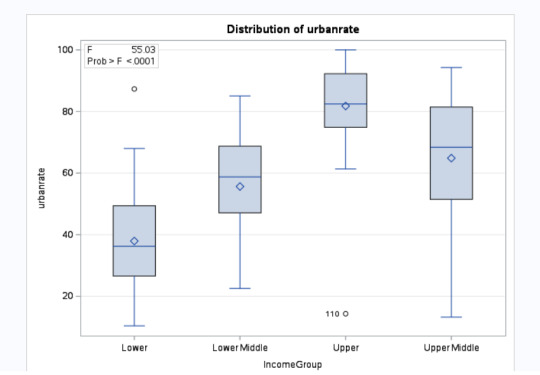
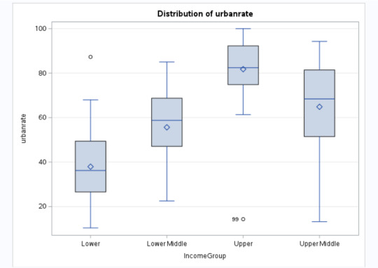
Proc Anova Data=Gapminder; Class IncomeGroup; Model urbanrate=IncomeGroup; Means IncomeGroup / Duncan; Where IncomeGroup NE 'NA'; Run;

Since the Gapminder dataset provided has quantitative variables, the variables incomeperperson, polityscore and urbanrate have been turned into categorical variables IncomeGroup, PoliticalStability and Urbanization respectively.

Anova Test

Proc Anova Data=Gapminder; Class IncomeGroup; Model urbanrate=IncomeGroup; Means IncomeGroup / Duncan; Where IncomeGroup NE 'NA'; Run;

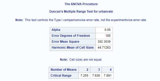
Through ANOVA we want to explore the statistical significance of the categorical variable IncomeGroup on the quantitative response variable urbanrate. The Post Hoc Test Comparison used was DUNCAN.

Null Hypothesis: There is no relationship between Income levels and urbanization in a country.

Alternate Hypothesis: There is a relationship between Income levels and urbanization in a country.

Results Screenshots

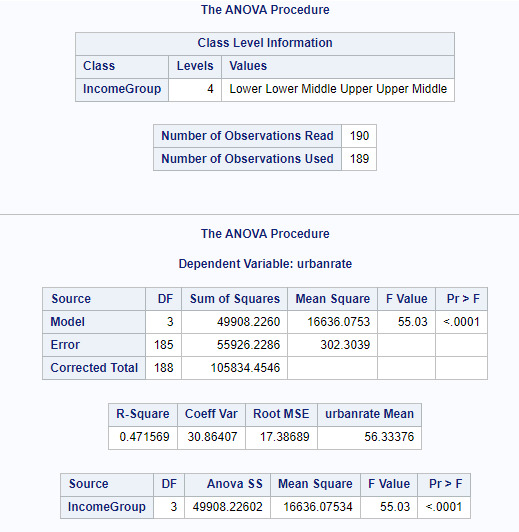
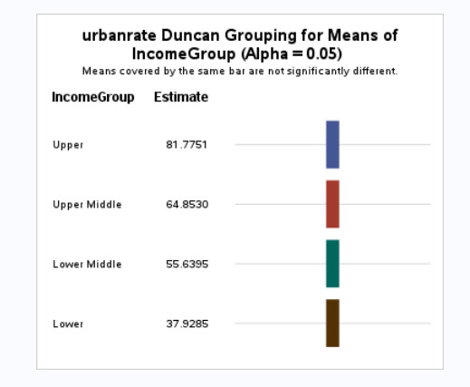
Explanation:

Since the p <0.05, we can reject the null hypothesis and say that there is a relationship between IncomeGroup and Urbanrate. Further studying, we see that higher the income, higher is the urbanization. The IncomeGroups Lower, Lower Middle, Upper Middle and Upper are statistically different when compared against Urbanization.