statsmaths - Tumblr blog

statsmaths · 3 years ago

Text

Assignment 4 - Data Visualization

import pandas import numpy import seaborn import matplotlib.pyplot as plt

data = pandas.read_csv('gapminder.csv', low_memory=False)

data = data.replace(r'^\s*$', numpy.NaN, regex=True)

#setting variables you will be working with to numeric

data['internetuserate'] = pandas.to_numeric(data['internetuserate']) data['urbanrate'] = pandas.to_numeric(data['urbanrate']) data['incomeperperson'] = pandas.to_numeric(data['incomeperperson']) data['hivrate'] = pandas.to_numeric(data['hivrate'])

desc1 = data['urbanrate'].describe()

#The below are descriptive statistics results for all the 2 variables used in the code

print (desc1)

count 203.000000

mean 56.769360

std 23.844933

min 10.400000

25% 36.830000

50% 57.940000

75% 74.210000

max 100.000000

desc2 = data['internetuserate'].describe() print (desc2)

count 192.000000

mean 35.632716

std 27.780285

min 0.210066

25% 9.999604

50% 31.810121

75% 56.416046

max 95.638113

#basic scatterplot: Q->Q

scat1 = seaborn.regplot(x="urbanrate", y="internetuserate", fit_reg=False, data=data)

plt.xlabel('Urban Rate')

Text(0.5, 0, 'Urban Rate')

plt.ylabel('Internet Use Rate')

Text(0, 0.5, 'Internet Use Rate')

plt.title('Scatterplot for the Association Between Urban Rate and Internet Use Rate')

Text(0.5, 1.0, 'Scatterplot for the Association Between Urban Rate and Internet Use Rate')

scat2 = seaborn.regplot(x="urbanrate", y="internetuserate", data=data)

#scatterplot graph image cannot be attached here

plt.xlabel('Urban Rate')

Text(0.5, 0, 'Urban Rate')

plt.ylabel('Internet Use Rate')

Text(0, 0.5, 'Internet Use Rate')

plt.title('Scatterplot for the Association Between Urban Rate and Internet Use Rate')

Text(0.5, 1.0, 'Scatterplot for the Association Between Urban Rate and Internet Use Rate')

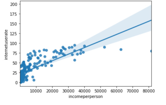
scat3 = seaborn.regplot(x="incomeperperson", y="internetuserate", data=data)

#scatterplot graph image cannot be attached here

plt.xlabel('Income per Person')

plt.ylabel('Internet Use Rate')

plt.title('Scatterplot for the Association Between Income per Person and Internet Use Rate')

scat4 = seaborn.regplot(x="incomeperperson", y="hivrate", data=data)

plt.xlabel('Income per Person')

plt.ylabel('HIV Rate')

plt.title('Scatterplot for the Association Between Income per Person and HIV Rate')

#quartile split (use qcut function & ask for 4 groups - gives you quartile split)

print ('Income per person - 4 categories - quartiles')

data['INCOMEGRP4']=pandas.qcut(data.incomeperperson, 4, labels=["1=25th%tile","2=50%tile","3=75%tile","4=100%tile"])

c10 = data['INCOMEGRP4'].value_counts(sort=False, dropna=True)

print(c10)

1=25th%tile 48

2=50%tile 47

3=75%tile 47

4=100%tile 48

#bivariate bar graph C->Q

seaborn.catplot(x='INCOMEGRP4', y='hivrate', data=data, kind="bar", ci=None)

#bar chart image cannot be attached here

plt.xlabel('income group')

plt.ylabel('mean HIV rate')

c11= data.groupby('INCOMEGRP4').size()

print (c11)

INCOMEGRP4

1=25th%tile 48

2=50%tile 47

3=75%tile 47

4=100%tile 48

#Summary:

We examined four variables - internateuser rate, urban rate, income per person and HIV rate from gapminder dataset and understand each variables descriptive statistics.

Next we did a co-relation analysis on these variables to find association b/w them. From the urban rate & internet use rate we find there is positive relation b/w them.

plt.xlabel('Urban Rate')

plt.ylabel('Internet Use Rate')

plt.title('Scatterplot for the Association Between Urban Rate and Internet Use Rate')

scat3 = seaborn.regplot(x="incomeperperson", y="internetuserate", data=data)

plt.xlabel('Income per Person')

plt.ylabel('Internet Use Rate')

plt.title('Scatterplot for the Association Between Income per Person and Internet Use Rate')

Text(0.5, 1.0, 'Scatterplot for the Association Between Income per Person and Internet Use Rate')

scat4 = seaborn.regplot(x="incomeperperson", y="hivrate", data=data)

plt.ylabel('HIV Rate')

plt.title('Scatterplot for the Association Between Income per Person and HIV Rate')

0 notes

statsmaths · 3 years ago

Text

Assignment 3

import pandas import numpy import statsmodels.formula.api as smf import statsmodels.stats.multicomp as multi

data = pandas.read_csv('gapminder.csv', low_memory=False)

print (len(data)) #number of observations (rows)

213

#setting variables you will be working with to numeric

data['urbanrate'] = pandas.to_numeric(data['urbanrate'], errors='coerce') data['femaleemployrate'] = pandas.to_numeric(data['femaleemployrate'], errors='coerce') data['lifeexpectancy'] = pandas.to_numeric(data['lifeexpectancy'], errors='coerce')

#creating three new variables for data management operations - urban,fer & le

data['urban']=data['urbanrate'] data['fer']=data['femaleemployrate'] data['le']=data['lifeexpectancy']

#data management for urbanrate

def urban (row): if row['urbanrate'] >= 75: return 3 if 25 <= row['urbanrate'] < 75: return 2 if row['urbanrate'] < 25: return 1

data['urban'] = data.apply(lambda row: urban (row),axis=1)

#frequency distribution for new varaibale urban

c1 = data['urban'].value_counts(sort=False) print (c1)

1.0 22

2.0 133

3.0 48

#data management for femaleemployrate

def fer (row): if row['femaleemployrate'] < 20: return 1 if 20 <= row['femaleemployrate'] < 40: return 2 if 40 <= row['femaleemployrate'] < 60: return 3 if 60 <= row['femaleemployrate'] < 80: return 4 if row['femaleemployrate'] >= 80: return 5

data['fer'] = data.apply(lambda row: fer (row),axis=1)

#frequency distribution for new varaibale fer

c2 = data['fer'].value_counts(sort=False) print (c2)

2.0 45

3.0 96

4.0 26

5.0 4

1.0 7

#data management for le

def le (row): if row['lifeexpectancy'] < 45: return 1 if 45 <= row['lifeexpectancy'] < 55: return 2 if 55 <= row['lifeexpectancy'] < 65: return 3 if 65 <= row['lifeexpectancy'] < 75: return 4 if row['lifeexpectancy'] >= 75: return 5

data['le'] = data.apply(lambda row: le (row),axis=1)

#frequency distribution for new varaibale le

c3 = data['le'].value_counts(sort=False) print (c3)

2.0 24

5.0 65

4.0 76

3.0 26

Summary:

In this module for data management I have collapsed the responses for urbanrate, femaleemployrate, and lifeexpectancy to create three new variables which are: urban, fer, and le.

For urban, the most commonly endorsed response was 2 (62.44%), meaning that most countries have an urban rate of 25% - 75%.

For fer, the most commonly endorsed response was 3 (45.07%), meaning that almost half of the countries have a female employment rate of 40% - 60%.

For le, the most commonly endorsed response was 4 (35.68%), meaning that the life expectancy in about one-third of the countries is 65 – 75 years old.

0 notes

statsmaths · 3 years ago

Text

Assignment 2 (week 2)

import pandas import numpy import statsmodels.formula.api as smf import statsmodels.stats.multicomp as multi

data = pandas.read_csv('gapminder.csv', low_memory=False)

print (len(data)) #number of observations (rows)

213

print (len(data.columns)) # number of variables (columns)

setting variables you will be working with to numeric

data['internetuserate'] = pandas.to_numeric(data['internetuserate'], errors='coerce') data['urbanrate'] = pandas.to_numeric(data['urbanrate'], errors='coerce') data['incomeperperson'] = pandas.to_numeric(data['incomeperperson'], errors='coerce')

ADDING TITLES (i.e. frequency distributions) for each variable

print ('counts for internetuserate - 2010 Internet users (per 100 people)') c1 = data['internetuserate'].value_counts(sort=False) print (c1)

counts for internetuserate - 2010 Internet users (per 100 people) 81.000000 1

66.000000 1

45.000000 1

65.000000 1

2.100213 1

36.000335 1

41.000128 1

33.616683 1

60.119707 1

1.699985 1

Name: internetuserate, Length: 192, dtype: int64

print ('percentages for internetuserate - 2010 Internet users (per 100 people)') p1 = data['internetuserate'].value_counts(sort=False, normalize=True) print (p1)

percentages for internetuserate - 2010 Internet users (per 100 people)

81.000000 0.005208

66.000000 0.005208

45.000000 0.005208

65.000000 0.005208

2.100213 0.005208

...

36.000335 0.005208

41.000128 0.005208

33.616683 0.005208

60.119707 0.005208

1.699985 0.005208

Name: internetuserate, Length: 192, dtype: float64

print ('counts for urbanrate - 2008 urban poplation (% of total)') c2 = data['urbanrate'].value_counts(sort=False) print(c2)

counts for urbanrate - 2008 urban poplation (% of total)

92.00 1

100.00 6

74.50 1

73.50 1 17.00 1

56.02 1

57.18 1

73.92 1

25.46 1

28.38 1

Name: urbanrate, Length: 194, dtype: int64

print ('percentages for urbanrate -2008 urban poplation (% of total)') p2 = data['urbanrate'].value_counts(sort=False, normalize=True) print (p2)

percentages for urbanrate -2008 urban poplation (% of total)

92.00 0.004926

100.00 0.029557

74.50 0.004926

73.50 0.004926

17.00 0.004926

...

56.02 0.004926

57.18 0.004926

73.92 0.004926

25.46 0.004926

28.38 0.004926

Name: urbanrate, Length: 194, dtype: float64

print ('counts for incomeperperson - 2010 GDP per capita in constant 2000 US $') c3 = data['incomeperperson'].value_counts(sort=False, dropna=False) print(c3)

counts for incomeperperson - 2010 GDP per capita in constant 2000 US $

NaN 23 8614.120219 1

39972.352768 1

279.180453 1

161.317137 1

377.421113 1

2344.896916 1

25306.187193 1

4180.765821 1

25575.352623 1

Name: incomeperperson, Length: 191, dtype: int64

print ('percentages for incomeperperson - 2010 GDP per capita in constant 2000 US $') p3 = data['incomeperperson'].value_counts(sort=False, normalize=True) print (p3)

percentages for incomeperperson - 2010 GDP per capita in constant 2000 US $

5188.900935 0.005263

8614.120219 0.005263

39972.352768 0.005263

279.180453 0.005263

161.317137 0.005263

...

377.421113 0.005263

2344.896916 0.005263

25306.187193 0.005263

4180.765821 0.005263

25575.352623 0.005263

Name: incomeperperson, Length: 190, dtype: float64

Summary: The data set taken here is 'gapminder.csv'. I have considered three variables of interest here which are:

internetuserate - 2010 Internet users (per 100 people)

urbanrate - 2008 urban poplation (% of total)

incomeperperson - 2010 GDP per capita in constant 2000 US $

The program is written and compiled in python and output snapshot is provided above. First I have run the # of observations in the data set (rows) which is 213. Then have run the # of variables in the data set (columns) whose value is 16.

Next, as per the assignment requirement, I have run the frequency distribution (i.e counts and percentages of all these three variables considered) and provided the snapshot.

0 notes

statsmaths · 3 years ago

Text

Assignment 1 - Data Management & Visualization

Data Set Selected: I would like to work on the Gapminder data set which contains data for all 192 UN members and which seeks to increase the use and understanding of statistics about social, economic, and environmental development at local, national, and global levels.

2. Research Question: Determine associations (if any) between "rate of internet users" by the "rate of the country's population living in urban settings".

Variables of interest from the codebook for the above stated hypothesis - Internetuserate & Urbanrate

Variables Type - Both are ordinal variables

3. Second hypothesis: Is there any association b/w rate of internet users and income per person for a region/country?

Variables of interest from the codebook for the above stated hypothesis - Internetuserate & Incomeperperson

Variables Type - Both are ordinal variables

4. Literature review of hypothesis #1: IJERPH | Free Full-Text | Association between Urban Upbringing and Compulsive Internet Use in Japan: A Cross-Sectional, Multilevel Study with Retrospective Recall (mdpi.com)

5. From the above literature review, the findings as are below:

Growing up in a large city was significantly associated with higher Compulsive Internet Use Scale (CIUS) scores (γ = 1.65, Standard Error (SE) = 0.45) and Mild CIU + Severe CIU (Exp(γ) = 1.44; 95% Confidence Interval (CI) (1.04–2.00)) compared to growing up in a small municipality

0 notes

statsmaths · 3 years ago

Text

Statistical Interactions - Assignment4

Objective:

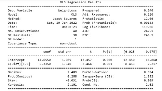
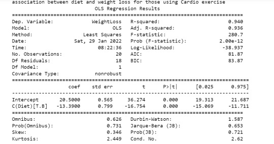
The goal of this assignment is to perform data analysis on a dataset ("diet_exercise.csv") to reveal any association that may exist b/w weight-loss and diet. Here the categorical variable is "Diet" given by two levels - Diet A & Diet B. The quantitative variable is weigh-tloss. The study is performed on these two variables using ANOVA method and results show below (first part) the p value is 0.00133 which is less than 0.05 which means there is slight significance b/w these two variables.

Now as part of this exercise we also wanted to introduce a moderator variable called "exercise" which has two levels - Cardio & Weights.

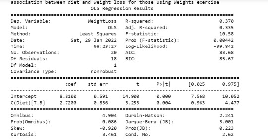
We ran the same tests with the introduction of the third moderator variable called "exercise" and found the below results.

Results:

The weight loss was shown to be significant for subjects who were on cardio exercise (p value of 2.00e-12) compared to those who used weights (p value of 0.00442). Hence the moderator variable is useful to show the actual relationship b/w two variables may be due to a 3rd moderator variable.

Code Snippet & Output:

import numpy

import pandas

import statsmodels.formula.api as smf

import statsmodels.stats.multicomp as multi

import seaborn

import matplotlib.pyplot as plt

data = pandas.read_csv('diet_exercise.csv', low_memory=False)

model1 = smf.ols(formula='WeightLoss ~ C(Diet)', data=data).fit()

print (model1.summary())

sub1 = data[['WeightLoss', 'Diet']].dropna()

m1= sub1.groupby('Diet').mean()

print ("means for WeightLoss by Diet A vs. B")

print (m1)

means for WeightLoss by Diet A vs. B

WeightLoss

Diet

A 14.655

B 9.320

st1= sub1.groupby('Diet').std()

print ("standard deviation for mean WeightLoss by Diet A vs. B")

print (st1)

standard deviation for mean WeightLoss by Diet A vs. B

WeightLoss

Diet

A 6.302086

B 2.779360

# bivariate bar graph

seaborn.factorplot(x="Diet", y="WeightLoss", data=data, kind="bar", ci=None)

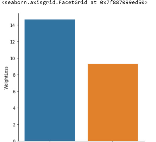
plt.xlabel('Diet Type')

plt.ylabel('Mean Weight Loss in pounds')

sub2=data[(data['Exercise']=='Cardio')]

sub3=data[(data['Exercise']=='Weights')]

model2 = smf.ols(formula='WeightLoss ~ C(Diet)', data=sub2).fit()

print ('association between diet and weight loss for those using Cardio exercise')

print (model2.summary())

model3 = smf.ols(formula='WeightLoss ~ C(Diet)', data=sub3).fit()

print ('association between diet and weight loss for those using Weights exercise')

print (model3.summary())

m3= sub2.groupby('Diet').mean()

print ("means for WeightLoss by Diet A vs. B for CARDIO")

print (m3)

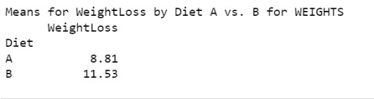
m4 = sub3.groupby('Diet').mean()

print ("Means for WeightLoss by Diet A vs. B for WEIGHTS")

print (m4)

0 notes

statsmaths · 3 years ago

Text

Assignment 3 - Calculating a Correlation Co-efficient (r):

Objective:

For this assignment we needed to generate a correlation coefficient from our data among the variables of interest. In this study we were interested to see if there was any association between 'Urban rate' & 'Internet use rate' as well as 'Income per person' & 'Internet use rate'. All three data sets are quantitative. Python was used to conduct the analysis.

Results:

1) Urban rate & internet use rate: r (Correlation coefficient) = 0.62 and P value = 4.540316299446745e-21. Since the r value is close to 1 and the p value is very small, this tells us that the relationship is statistically significant between urbanization rate and internet use rate.

2) Income per person & internet use rate: r (Correlation coefficient) = 0.75 and P value = 3.067338031233027e-34. Since the r value is close to 1 and the p value is very small, this tells us that the relationship is statistically significant between income per person and internet use rate.

Code Snippet:

import pandas

import numpy

import seaborn

import scipy

import matplotlib.pyplot as plt

data = pandas.read_csv('gapminder.csv', low_memory=False)

#setting variables you will be working with to numeric

data['internetuserate'] = pandas.to_numeric(data['internetuserate'], errors='coerce')

data['urbanrate'] = pandas.to_numeric(data['urbanrate'], errors='coerce')

data['incomeperperson'] = pandas.to_numeric(data['incomeperperson'], errors='coerce')

data['incomeperperson']=data['incomeperperson'].replace(' ', numpy.nan)

scat1 = seaborn.regplot(x="urbanrate", y="internetuserate", fit_reg=True, data=data)

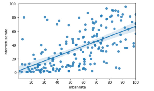
plt.xlabel('Urban Rate')

plt.ylabel('Internet Use Rate')

plt.title('Scatterplot for the Association Between Urban Rate and Internet Use Rate')

scat2 = seaborn.regplot(x="incomeperperson", y="internetuserate", fit_reg=True, data=data)

plt.xlabel('Income per Person')

plt.ylabel('Internet Use Rate')

plt.title('Scatterplot for the Association Between Income per Person and Internet Use Rate')

data_clean=data.dropna()

print ('association between urbanrate and internetuserate')

print (scipy.stats.pearsonr(data_clean['urbanrate'], data_clean['internetuserate']))

association between urbanrate and internetuserate

(0.6244640029489794, 4.540316299446745e-21)

print ('association between incomeperperson and internetuserate')

print (scipy.stats.pearsonr(data_clean['incomeperperson'], data_clean['internetuserate']))

association between incomeperperson and internetuserate (0.7507274333051273, 3.067338031233027e-34)

0 notes

statsmaths · 3 years ago

Text

Assignment 2

Objective:

For this assignment a Chi-square Test of Independence in Python was supposed to be executed to analyze association b/w two categorical variables - 'Nicotine Dependence' & 'Days smoked per month'. The dataset "NESACR.csv" was used to see if there is an association b/w nicotine dependence proportion & cigarettes smoked per month for young adults in age bracket of 18 to 25. In other words if there is an increase in nicotine dependence when the # of cigarettes smoked in a month increased. There were six levels for the cigarettes smoked per month - 1, 2.5, 6, 14, 22 & 30. We did run a post-hoc analysis b/w each of the pairs i.e nicotine dependence within each smoking frequency group.

Results:

The results shows the p value is significant when the # cigarettes smoked increased. The chi-square value, p value & expected counts for each smoking frequency group is shown below.

Code Snippet & Output:

import pandas

import numpy

import scipy.stats

import seaborn

import matplotlib.pyplot as plt

data = pandas.read_csv('nesarc.csv', low_memory=False)

# new code setting variables you will be working with to numeric

data['TAB12MDX'] = pandas.to_numeric(data['TAB12MDX'], errors='coerce')

data['CHECK321'] = pandas.to_numeric(data['CHECK321'], errors='coerce')

data['S3AQ3B1'] = pandas.to_numeric(data['S3AQ3B1'], errors='coerce')

data['S3AQ3C1'] = pandas.to_numeric(data['S3AQ3C1'], errors='coerce')

data['AGE'] = pandas.to_numeric(data['AGE'], errors='coerce')

#subset data to young adults age 18 to 25 who have smoked in the past 12 months

sub1=data[(data['AGE']>=18) & (data['AGE']<=25) & (data['CHECK321']==1)]

#make a copy of my new subsetted data

sub2 = sub1.copy()

# recode missing values to python missing (NaN)

sub2['S3AQ3B1']=sub2['S3AQ3B1'].replace(9, numpy.nan)

sub2['S3AQ3C1']=sub2['S3AQ3C1'].replace(99, numpy.nan)

#recoding values for S3AQ3B1 into a new variable, USFREQMO

recode1 = {1: 30, 2: 22, 3: 14, 4: 6, 5: 2.5, 6: 1}

sub2['USFREQMO']= sub2['S3AQ3B1'].map(recode1)

# contingency table of observed counts

ct1=pandas.crosstab(sub2['TAB12MDX'], sub2['USFREQMO'])

print (ct1)

USFREQMO 1.0 2.5 6.0 14.0 22.0 30.0

TAB12MDX

0 64 53 69 59 41 521

1 7 12 19 32 27 799

# column percentages

colsum=ct1.sum(axis=0)

colpct=ct1/colsum

print(colpct)

USFREQMO 1.0 2.5 6.0 14.0 22.0 30.0

TAB12MDX

0 0.901408 0.815385 0.784091 0.648352 0.602941 0.394697

1 0.098592 0.184615 0.215909 0.351648 0.397059 0.605303

# chi-square

print ('chi-square value, p value, expected counts')

cs1= scipy.stats.chi2_contingency(ct1)

print (cs1)

chi-square value, p value, expected counts

(165.27320708055845, 7.436364208390599e-34, 5, array([[ 33.64474457, 30.80152672, 41.70052848, 43.1221374 , 32.22313564, 625.50792719], [ 37.35525543, 34.19847328, 46.29947152, 47.8778626 , 35.77686436, 694.49207281]]))

# set variable types

sub2["USFREQMO"] = sub2["USFREQMO"].astype('category')

sub2['TAB12MDX'] = pandas.to_numeric(sub2['TAB12MDX'], errors='coerce')

# graph percent with nicotine dependence within each smoking frequency group

seaborn.factorplot(x="USFREQMO", y="TAB12MDX", data=sub2, kind="bar", ci=None)

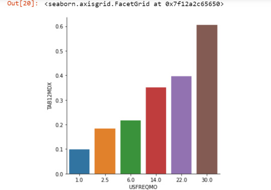
plt.xlabel('Days smoked per month')

plt.ylabel('Proportion Nicotine Dependent')

recode2 = {1: 1, 2.5: 2.5}

sub2['COMP1v2']= sub2['USFREQMO'].map(recode2)

ct2=pandas.crosstab(sub2['TAB12MDX'], sub2['COMP1v2'])

print (ct2)

COMP1v2 1.0 2.5

TAB12MDX

0 64 53

1 7 12

# column percentages

colsum=ct2.sum(axis=0)

colpct=ct2/colsum

print(colpct)

COMP1v2 1.0 2.5

TAB12MDX

0 0.901408 0.815385

1 0.098592 0.184615

print ('chi-square value, p value, expected counts')

cs2= scipy.stats.chi2_contingency(ct2)

print (cs2)

chi-square value, p value, expected counts

(1.4348930637007287, 0.2309675448977717, 1, array([[61.08088235, 55.91911765], [ 9.91911765, 9.08088235]]))

recode3 = {1: 1, 6: 6}

sub2['COMP1v6']= sub2['USFREQMO'].map(recode3)

# contingency table of observed counts

ct3=pandas.crosstab(sub2['TAB12MDX'], sub2['COMP1v6'])

print (ct3)

COMP1v6 1.0 6.0

TAB12MDX

0 64 69

1 7 19

# column percentages

colsum=ct3.sum(axis=0)

colpct=ct3/colsum

print(colpct)

COMP1v6 1.0 6.0

TAB12MDX

0 0.901408 0.784091

1 0.098592 0.215909

print ('chi-square value, p value, expected counts')

cs3= scipy.stats.chi2_contingency(ct3)

print (cs3)

chi-square value, p value, expected counts

(3.142840191220936, 0.07626090198286821, 1, array([[59.38993711, 73.61006289], [11.61006289, 14.38993711]]))

recode4 = {1: 1, 14: 14}

sub2['COMP1v14']= sub2['USFREQMO'].map(recode4)

# contingency table of observed counts

ct4=pandas.crosstab(sub2['TAB12MDX'], sub2['COMP1v14'])

print (ct4)

COMP1v14 1.0 14.0

TAB12MDX

0 64 59

1 7 32

# column percentages

colsum=ct4.sum(axis=0)

colpct=ct4/colsum

print(colpct)

COMP1v14 1.0 14.0

TAB12MDX

0 0.901408 0.648352

1 0.098592 0.351648

print ('chi-square value, p value, expected counts')

cs4= scipy.stats.chi2_contingency(ct4)

print (cs4)

chi-square value, p value, expected counts

(12.622564075461572, 0.00038111819882681824, 1, array([[53.90740741, 69.09259259], [17.09259259, 21.90740741]]))

recode5 = {1: 1, 22: 22}

sub2['COMP1v22']= sub2['USFREQMO'].map(recode5)

# contingency table of observed counts

ct5=pandas.crosstab(sub2['TAB12MDX'], sub2['COMP1v22'])

print (ct5)

COMP1v22 1.0 22.0

TAB12MDX

0 64 41

1 7 27

# column percentages

colsum=ct5.sum(axis=0)

colpct=ct5/colsum

print(colpct)

COMP1v22 1.0 22.0

TAB12MDX

0 0.901408 0.602941

1 0.098592 0.397059

print ('chi-square value, p value, expected counts')

cs5= scipy.stats.chi2_contingency(ct5)

print (cs5)

chi-square value, p value, expected counts

(15.169488833230059, 9.827865291318501e-05, 1, array([[53.63309353, 51.36690647], [17.36690647, 16.63309353]]))

recode6 = {1: 1, 30: 30}

sub2['COMP1v30']= sub2['USFREQMO'].map(recode6)

# contingency table of observed counts

ct6=pandas.crosstab(sub2['TAB12MDX'], sub2['COMP1v30'])

print (ct6)

COMP1v30 1.0 30.0

TAB12MDX

0 64 521

1 7 799

# column percentages

colsum=ct6.sum(axis=0)

colpct=ct6/colsum

print(colpct)

COMP1v30 1.0 30.0

TAB12MDX

0 0.901408 0.394697

1 0.098592 0.605303

print ('chi-square value, p value, expected counts')

cs6= scipy.stats.chi2_contingency(ct6)

print (cs6)

chi-square value, p value, expected counts

(68.92471874488487, 1.0229460827061155e-16, 1, array([[ 29.85981308, 555.14018692], [ 41.14018692, 764.85981308]]))

recode7 = {2.5: 2.5, 6: 6}

sub2['COMP2v6']= sub2['USFREQMO'].map(recode7)

# contingency table of observed counts

ct7=pandas.crosstab(sub2['TAB12MDX'], sub2['COMP2v6'])

print (ct7)

COMP2v6 2.5 6.0

TAB12MDX

0 53 69

1 12 19

# column percentages

colsum=ct7.sum(axis=0)

colpct=ct7/colsum

print(colpct)

COMP2v6 2.5 6.0

TAB12MDX

0 0.815385 0.784091

1 0.184615 0.215909

print ('chi-square value, p value, expected counts')

cs7=scipy.stats.chi2_contingency(ct7)

print (cs7)

chi-square value, p value, expected counts (0.07430561076945266, 0.7851679729700605, 1, array([[51.83006536, 70.16993464], [13.16993464, 17.83006536]]))

0 notes

statsmaths · 3 years ago

Text

Assignment 1

import numpy import pandas import statsmodels.formula.api as smf import statsmodels.stats.multicomp as multi

data = pandas.read_csv('nesarc.csv', low_memory=False)

#setting variables you will be working with to numeric data['S3AQ3B1'] = pandas.to_numeric(data['S3AQ3B1'], errors='coerce') data['S3AQ3C1'] = pandas.to_numeric(data['S3AQ3C1'], errors='coerce') data['CHECK321'] = pandas.to_numeric(data['CHECK321'], errors='coerce')

#subset data to young adults age 18 to 25 who have smoked in the past 12 months sub1=data[(data['AGE']>=18) & (data['AGE']<=25) & (data['CHECK321']==1)]

#SETTING MISSING DATA sub1['S3AQ3B1']=sub1['S3AQ3B1'].replace(9, numpy.nan) sub1['S3AQ3C1']=sub1['S3AQ3C1'].replace(99, numpy.nan)

#recoding number of days smoked in the past month recode1 = {1: 30, 2: 22, 3: 14, 4: 5, 5: 2.5, 6: 1} sub1['USFREQMO']= sub1['S3AQ3B1'].map(recode1)

#converting new variable USFREQMMO to numeric sub1['USFREQMO'] = pandas.to_numeric(sub1['USFREQMO'], errors='coerce')

# Creating a secondary variable multiplying the days smoked/month and the number of cig/per day sub1['NUMCIGMO_EST']=sub1['USFREQMO'] * sub1['S3AQ3C1'] sub1['NUMCIGMO_EST']= pandas.to_numeric(sub1['NUMCIGMO_EST'], errors='coerce')

ct1 = sub1.groupby('NUMCIGMO_EST').size() print (ct1)

NUMCIGMO_EST

1.0 29

2.0 14

2.5 11

3.0 12

4.0 2

1050.0 1

1200.0 29

1800.0 2

2400.0 1

2940.0 1

Length: 66, dtype: int64

# using ols function for calculating the F-statistic and associated p value model1 = smf.ols(formula='NUMCIGMO_EST ~ C(MAJORDEPLIFE)', data=sub1) results1 = model1.fit() print (results1.summary())

OLS Regression Results ================================================

Dep. Variable: NUMCIGMO_EST R-squared: 0.002

Model: OLS Adj. R-squared: 0.002

Method: Least Squares F-statistic: 3.550

Date: Wed, 26 Jan 2022 Prob (F-statistic): 0.0597

Time: 17:58:07 Log-Likelihood: -11934.

No. Observations: 1697 AIC: 2.387e+04

Df Residuals: 1695 BIC: 2.388e+04

Df Model: 1

Covariance Type: nonrobust ================================================

coef std err t P>|t| [0.025 0.975]

------------------------------------------------------------------------------

Intercept 312.8380 7.747 40.381 0.000 297.643 328.033

C(MAJORDEPLIFE)[T.1] 28.5370 15.146 1.884 0.060 -1.169 58.243 ================================================

Omnibus: 673.875 Durbin-Watson: 1.982

Prob(Omnibus): 0.000 Jarque-Bera (JB): 5043.141

Skew: 1.672 Prob(JB): 0.00

Kurtosis: 10.755 Cond. No. 2.46 ================================================

Warnings: [1] Standard Errors assume that the covariance matrix of the errors is correctly specified.

sub2 = sub1[['NUMCIGMO_EST', 'MAJORDEPLIFE']].dropna()

print ('means for numcigmo_est by major depression status') m1= sub2.groupby('MAJORDEPLIFE').mean() print (m1)

means for numcigmo_est by major depression status

NUMCIGMO_EST

MAJORDEPLIFE

0 312.837989

1 341.375000

print ('standard deviations for numcigmo_est by major depression status') sd1 = sub2.groupby('MAJORDEPLIFE').std() print (sd1)

standard deviations for numcigmo_est by major depression status NUMCIGMO_EST

MAJORDEPLIFE

0 269.002344

1 288.495118 sub3 = sub1[['NUMCIGMO_EST', 'ETHRACE2A']].dropna()

model2 = smf.ols(formula='NUMCIGMO_EST ~ C(ETHRACE2A)', data=sub3).fit() print (model2.summary())

OLS Regression Results ================================================

Dep. Variable: NUMCIGMO_EST R-squared: 0.055

Model: OLS Adj. R-squared: 0.052

Method: Least Squares F-statistic: 24.40

Date: Wed, 26 Jan 2022 Prob (F-statistic): 1.18e-19

Time: 18:01:14 Log-Likelihood: -11888.

No. Observations: 1697 AIC: 2.379e+04

Df Residuals: 1692 BIC: 2.381e+04

Df Model: 4

Covariance Type: nonrobust ============================================================

coef std err t P>|t| [0.025 0.975]

-------------------------------------------------------------------------------------

Intercept 368.7865 8.229 44.814 0.000 352.646 384.927 C(ETHRACE2A)[T.2] -109.5127 20.189 -5.424 0.000 -149.111 -69.914 C(ETHRACE2A)[T.3] -57.7984 42.038 -1.375 0.169 -140.250 24.653 C(ETHRACE2A)[T.4] -124.5279 36.033 -3.456 0.001 -195.201 -53.854 C(ETHRACE2A)[T.5] -149.0283 16.795 -8.873 0.000 -181.969 -116.087 ============================================================ Omnibus: 712.397 Durbin-Watson: 1.994

Prob(Omnibus): 0.000 Jarque-Bera (JB): 6548.614

Skew: 1.717 Prob(JB): 0.00

Kurtosis: 11.990 Cond. No. 6.72 ============================================================Warnings: [1] Standard Errors assume that the covariance matrix of the errors is correctly specified.

print ('means for numcigmo_est by major depression status') m2= sub3.groupby('ETHRACE2A').mean() print (m2)

means for numcigmo_est by major depression status

NUMCIGMO_EST

ETHRACE2A

1 368.786528

2 259.273810

3 310.988095

4 244.258621

5 219.758258

print ('standard deviations for numcigmo_est by major depression status') sd2 = sub3.groupby('ETHRACE2A').std() print (sd2)

standard deviations for numcigmo_est by major depression status NUMCIGMO_EST

ETHRACE2A

1 281.430730

2 278.677392

3 260.116964

4 195.076441

5 220.859365

mc1 = multi.MultiComparison(sub3['NUMCIGMO_EST'], sub3['ETHRACE2A']) res1 = mc1.tukeyhsd() print(res1.summary())

Multiple Comparison of Means - Tukey HSD, FWER=0.05 ========================================================= group1 group2 meandiff p-adj lower upper reject

----- ---------------------------------------------------------

1 2 -109.5127 0.001 -164.6441 -54.3814 True

1 3 -57.7984 0.6251 -172.5914 56.9945 False

1 4 -124.5279 0.0051 -222.9229 -26.1329 True

1 5 -149.0283 0.001 -194.89 -103.1665 True

2 3 51.7143 0.7555 -71.6021 175.0307 False

2 4 -15.0152 0.9 -123.233 93.2026 False

2 5 -39.5156 0.4492 -103.8025 24.7714 False

3 4 -66.7295 0.7058 -214.5437 81.0848 False

3 5 -91.2298 0.2269 -210.6902 28.2305 False

4 5 -24.5004 0.9 -128.3027 79.302 False

---------------------------------------------------------

1 note · View note