stattp-blog1 - Tumblr blog

stattp-blog1 · 6 years ago

Text

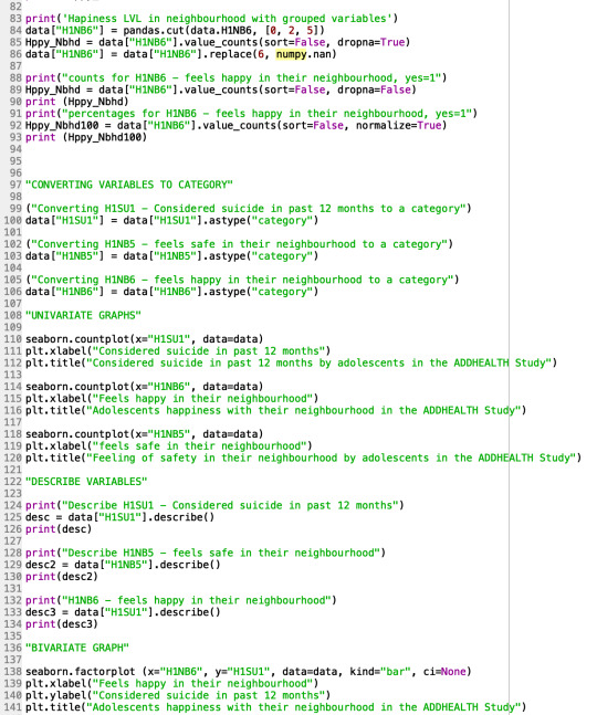
Running a Classification Tree

CODE:

#!/usr/bin/env python3 # -*- coding: utf-8 -*- """ Created on Sun Dec 1 15:34:18 2019

""" from pandas import Series, DataFrame import pandas as pd import numpy as np import os import matplotlib.pylab as plt from sklearn.model_selection import train_test_split from sklearn.tree import DecisionTreeClassifier from sklearn.metrics import classification_report import sklearn.metrics

""" Data Engineering and Analysis """ #Load the dataset

AH_data = pd.read_csv("/Users/tyler2k/Downloads/Data Analysis Course/addhealth_pds.csv")

data_clean = AH_data.dropna()

data_clean.dtypes data_clean.describe()

""" Modeling and Prediction """ #Split into training and testing sets

predictors = data_clean[['H1SU1', 'H1SU2', 'H1NB5', 'H1NB6']]

targets = data_clean.H1SU3

pred_train, pred_test, tar_train, tar_test = train_test_split(predictors, targets, test_size=.4)

pred_train.shape pred_test.shape tar_train.shape tar_test.shape

#Build model on training data classifier=DecisionTreeClassifier() classifier=classifier.fit(pred_train,tar_train)

predictions=classifier.predict(pred_test)

sklearn.metrics.confusion_matrix(tar_test,predictions) sklearn.metrics.accuracy_score(tar_test, predictions)

#Displaying the decision tree #from sklearn import tree #from StringIO import StringIO #from io import BytesIO as StringIO #from StringIO import StringIO #from IPython.display import Image #out = StringIO() #tree.export_graphviz(classifier, out_file=out) #import pydotplus #graph=pydotplus.graph_from_dot_data(out.getvalue()) #Image(graph.create_png())

#Displaying the decision tree

from sklearn import tree

#from StringIO import StringIO

from io import StringIO

#from StringIO import StringIO

from IPython.display import display, Image

out = StringIO()

tree.export_graphviz(classifier, out_file=out,

feature_names=predictors.columns,

filled=True, rounded=True,

special_characters=True,

proportion = True)

import pydotplus

print(out.getvalue())

graph=pydotplus.graph_from_dot_data(out.getvalue())

# Display inline image of Tree - Inline image is not useful

Img=(Image(graph.create_png()))

display(Img)

#Write image to file so it can be rotated and expanded

graph.write_png('MyfileNameTreeChart.png')

Output:

runfile('/Users/Downloads/Data Analysis Course/Course 4 Week 1', wdir='/Users//Downloads/Data Analysis Course') Reloaded modules: __mp_main__ /Users/tyler2k/Downloads/Data Analysis Course/Course 4 Week 1:1: DtypeWarning: Columns (8,11,22,65,134,135,177,205,206,207,208,346,366,523,532,533,753,755,756,842,843,847,848,849,856,885,886,887,888,889,890,891,892,893,894,895,896,897,898,899,900,901,902,903,904,905,906,908,909,910,911,912,913,914,915,916,917,918,919,920,921,922,923,924,925,926,927,928,929,930,931,932,933,934,935,936,937,938,939,940,941,942,943,944,945,946,966,967,974,979,980,982,986,987,989,991,992,994,1010,1035,1036,1037,1038,1039,1040,1041,1042,1043,1044,1045,1046,1047,1048,1049,1050,1051,1052,1053,1073,1075,1078,1079,1080,1081,1084,1085,1086,1087,1088,1091,1092,1093,1094,1095,1097,1098,1099,1119,1141,1142,1143,1144,1145,1146,1147,1148,1149,1150,1151,1152,1153,1154,1155,1156,1157,1158,1159,1160,1161,1162,1163,1164,1184,1185,1186,1187,1190,1191,1192,1193,1194,1197,1198,1199,1200,1201,1219,1221,1222,1235,1236,1237,1238,1239,1240,1262,1263,1264,1265,1266,1267,1268,1269,1270,1271,1272,1273,1274,1275,1276,1277,1278,1279,1280,1281,1282,1283,1284,1285,1286,1300,1302,1383,1384,1389,1390,1406,1407,1408,1409,1410,1411,1433,1434,1435,1436,1437,1438,1439,1440,1441,1442,1443,1444,1445,1446,1447,1448,1449,1450,1451,1452,1453,1454,1455,1456,1457,1458,1459,1460,1476,1477,1478,1479,1482,1483,1484,1485,1486,1489,1490,1491,1492,1493,1554,1555,1582,1604,1605,1606,1607,1608,1609,1610,1611,1612,1613,1614,1615,1616,1617,1618,1619,1620,1621,1622,1623,1624,1625,1626,1627,1628,1629,1630,1631,1632,1633,1634,1635,1636,1637,1638,1639,1647,1648,1649,1650,1653,1654,1655,1656,1657,1660,1661,1662,1663,1664,1725,1726,1757,1758,1759,1785,1786,1787,1788,1789,1790,1791,1792,1793,1794,1795,1796,1797,1875,1876,1877,1885,1886,1887,2011,2012,2013,2021,2022,2023,2024,2025,2026,2027,2028,2029,2030,2031,2032,2033,2034,2120,2121,2122,2123,2124,2125,2126,2127,2128,2129,2130,2131,2132,2133,2134,2135,2136,2137,2138,2139,2140,2141,2142,2143,2144,2145,2146,2147,2148,2149,2150,2151,2152,2153,2154,2155,2156,2157,2158,2159,2160,2161,2162,2163,2164,2165,2166,2167,2168,2169,2170,2171,2172,2173,2174,2175,2176,2177,2178,2179,2180,2181,2182,2183,2184,2185,2186,2187,2188,2189,2190,2191,2192,2193,2194,2195,2196,2197,2198,2199,2200,2201,2202,2203,2204,2205,2206,2207,2208,2209,2210,2211,2212,2213,2214,2215,2216,2217,2218,2219,2220,2221,2222,2223,2224,2225,2226) have mixed types. Specify dtype option on import or set low_memory=False. #!/usr/bin/env python3 digraph Tree { node [shape=box, style="filled, rounded", color="black", fontname=helvetica] ; edge [fontname=helvetica] ; 0 [label=<H1SU1 ≤ 0.5 gini = 0.228 samples = 100.0% value = [0.091, 0.019, 0.012, 0.002, 0.003, 0.001, 0.873]>, fillcolor="#e53986db"] ; 1 [label=<gini = 0.0 samples = 86.3% value = [0.0, 0.0, 0.0, 0.0, 0.0, 0.0, 1.0]>, fillcolor="#e53986ff"] ; 0 -> 1 [labeldistance=2.5, labelangle=45, headlabel="True"] ; 2 [label=<H1SU1 ≤ 3.5 gini = 0.527 samples = 13.7% value = [0.663, 0.14, 0.084, 0.011, 0.022, 0.004, 0.075]>, fillcolor="#e581399b"] ; 0 -> 2 [labeldistance=2.5, labelangle=-45, headlabel="False"] ; 3 [label=<H1NB6 ≤ 2.5 gini = 0.454 samples = 12.7% value = [0.717, 0.152, 0.091, 0.012, 0.024, 0.004, 0.0]>, fillcolor="#e58139aa"] ; 2 -> 3 ; 4 [label=<H1NB6 ≤ 1.5 gini = 0.591 samples = 1.9% value = [0.6, 0.173, 0.107, 0.067, 0.053, 0.0, 0.0]>, fillcolor="#e5813984"] ; 3 -> 4 ; 5 [label=<H1NB5 ≤ 0.5 gini = 0.609 samples = 0.7% value = [0.552, 0.276, 0.034, 0.069, 0.069, 0.0, 0.0]>, fillcolor="#e5813961"] ; 4 -> 5 ; 6 [label=<gini = 0.565 samples = 0.5% value = [0.6, 0.25, 0.0, 0.05, 0.1, 0.0, 0.0]>, fillcolor="#e5813977"] ; 5 -> 6 ; 7 [label=<gini = 0.667 samples = 0.2% value = [0.444, 0.333, 0.111, 0.111, 0.0, 0.0, 0.0]>, fillcolor="#e581392a"] ; 5 -> 7 ; 8 [label=<H1NB5 ≤ 0.5 gini = 0.561 samples = 1.2% value = [0.63, 0.109, 0.152, 0.065, 0.043, 0.0, 0.0]>, fillcolor="#e5813990"] ; 4 -> 8 ; 9 [label=<gini = 0.625 samples = 0.5% value = [0.55, 0.2, 0.1, 0.15, 0.0, 0.0, 0.0]>, fillcolor="#e5813970"] ; 8 -> 9 ; 10 [label=<gini = 0.476 samples = 0.7% value = [0.692, 0.038, 0.192, 0.0, 0.077, 0.0, 0.0]>, fillcolor="#e581399e"] ; 8 -> 10 ; 11 [label=<H1NB5 ≤ 0.5 gini = 0.426 samples = 10.7% value = [0.737, 0.148, 0.088, 0.002, 0.019, 0.005, 0.0]>, fillcolor="#e58139b0"] ; 3 -> 11 ; 12 [label=<H1NB6 ≤ 3.5 gini = 0.396 samples = 1.3% value = [0.76, 0.08, 0.14, 0.0, 0.02, 0.0, 0.0]>, fillcolor="#e58139b8"] ; 11 -> 12 ; 13 [label=<gini = 0.462 samples = 0.9% value = [0.706, 0.088, 0.176, 0.0, 0.029, 0.0, 0.0]>, fillcolor="#e58139a4"] ; 12 -> 13 ; 14 [label=<H1NB6 ≤ 4.5 gini = 0.227 samples = 0.4% value = [0.875, 0.062, 0.062, 0.0, 0.0, 0.0, 0.0]>, fillcolor="#e58139dd"] ; 12 -> 14 ; 15 [label=<gini = 0.292 samples = 0.3% value = [0.833, 0.083, 0.083, 0.0, 0.0, 0.0, 0.0]>, fillcolor="#e58139d1"] ; 14 -> 15 ; 16 [label=<gini = 0.0 samples = 0.1% value = [1.0, 0.0, 0.0, 0.0, 0.0, 0.0, 0.0]>, fillcolor="#e58139ff"] ; 14 -> 16 ; 17 [label=<H1NB5 ≤ 4.5 gini = 0.429 samples = 9.5% value = [0.734, 0.157, 0.081, 0.003, 0.019, 0.005, 0.0]>, fillcolor="#e58139af"] ; 11 -> 17 ; 18 [label=<H1NB6 ≤ 3.5 gini = 0.431 samples = 9.4% value = [0.733, 0.158, 0.082, 0.003, 0.019, 0.005, 0.0]>, fillcolor="#e58139ae"] ; 17 -> 18 ; 19 [label=<gini = 0.393 samples = 2.6% value = [0.762, 0.139, 0.079, 0.0, 0.01, 0.01, 0.0]>, fillcolor="#e58139b9"] ; 18 -> 19 ; 20 [label=<H1NB6 ≤ 4.5 gini = 0.444 samples = 6.8% value = [0.722, 0.165, 0.083, 0.004, 0.023, 0.004, 0.0]>, fillcolor="#e58139aa"] ; 18 -> 20 ; 21 [label=<gini = 0.455 samples = 4.1% value = [0.714, 0.161, 0.093, 0.006, 0.019, 0.006, 0.0]>, fillcolor="#e58139a8"] ; 20 -> 21 ; 22 [label=<gini = 0.428 samples = 2.7% value = [0.733, 0.171, 0.067, 0.0, 0.029, 0.0, 0.0]>, fillcolor="#e58139ad"] ; 20 -> 22 ; 23 [label=<gini = 0.0 samples = 0.1% value = [1.0, 0.0, 0.0, 0.0, 0.0, 0.0, 0.0]>, fillcolor="#e58139ff"] ; 17 -> 23 ; 24 [label=<gini = 0.0 samples = 1.0% value = [0.0, 0.0, 0.0, 0.0, 0.0, 0.0, 1.0]>, fillcolor="#e53986ff"] ; 2 -> 24 ; }

Image: https://stattp.tumblr.com/post/189530701105/course-4-week-1

Summary:

My decision tree was based on the variable H1SU3 (Did any suicide attempt result in an injury, poisoning, or overdose that had to be treated by a doctor or nurse?). My branches were based on variables H1SU1 (During the past 12 months, did you ever seriously think about committing suicide?), H1SU2 (During the past 12 months, how many times did you actually attempt suicide?), H1NB5 (Do you usually feel safe in your neighborhood?), H1NB6 (On the whole, how happy are you with living in your neighborhood?).

0 notes

stattp-blog1 · 6 years ago

Photo

Course 4 week 1

0 notes

stattp-blog1 · 6 years ago

Text

Test a Logistic Regression Model

CODE

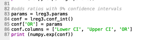
OUTPUT

When adjusting for the variable H1SU4 (whether the respondent had friends that attempted suicide within the last 12 months) I found that it had a strong impact on whether a respondent had attempt suicide (H1SU1) as the odds ratio was above 1 though (OR: 4.31, CI: 3.98-5.05, p:0)

When analyzing with the confounding variable H1SU5, which inquires whether the respondent’s friend succeeded in committing suicide, I found that H1SU4, whether the respondent had friends that attempted suicide within the last 12 months, was very significant to H1SU1 —whether a respondent had attempt suicide— due to a high odds ratio (OR: 82.7, CI: 8.47-806.81, p: 0).

These results support my hypothesis and also support the hypothesis that a person is much more likely to attempt suicide if a friend has attempted themselves, and even more so if they succeeded.

0 notes

stattp-blog1 · 6 years ago

Text

Test a Multiple Regression Model

I found in my regression analysis that my chosen explanatory variables (birth order, and level of happiness living in neighbourhood) have little correlation with my response variable (number of suicide attempts) especially, and not surprisingly, when controlling for birth order. For each of my regression tests on both explanatory variables, the p values were much higher than 0.05, with all of them being larger than 0.201; I thus cannot reject the null hypothesis. However, my beta coefficient values for birth order (Childpos) and happiness level in neighbourhood (Happylvl) were both negative signifying a linear association between my variables; my squared beta coefficient (Happylvl ** 2) was positive and therefore not linear.

These results do not support my hypothesis and I believe it is because I had to choose a third qualitative variable in a data set which mostly contains qualitative data. Thus, I had to choose a variable which was somewhat related to my other variables (birth order) to complete this exercise. I believe that I might have found stronger correlations if there was a greater choice of relevant quantitative variables in my dataset.

There was no evidence that my confounding variable (birth order) helped explain correlation between my two other variables. Already, both variables had a weak but present correlation between them; the addition of birth order did not improve the correlation and that is most likely due to the fact that it isn’t an entirely relevant variable to the two other

�� a) QQ PLOT

My qq plot is misshapen and demonstrates that my data and this model are not very compatible. Since my qq plot is not a straight line, it means that my model estimated residuals are not what would would be expected if the residuals were normally distributed.

b) Standardized Residuals

Many of my standard deviation residuals find themselves at 2 or higher meaning that the level of error in my model is unacceptable and that the model is a poor fit for my chosen data. This means that I need to include additional relevant variables to properly evaluate correlation.

c) Leverage plot

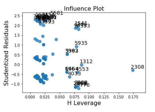
My influence plot shows many studentized residuals with high values, and a single value (2308) with a significantly high leverage.

CODE

OUTPUT

0 notes

stattp-blog1 · 6 years ago

Text

Test a Basic Linear Regression Model

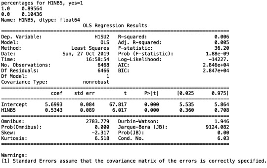
My regression analysis demonstrated that the number of suicide attempts (H1SU2) [Beta=5.6993, p=1.88e-09] is positively associated with respondents’ feeling of safety in their neighbourhoods. I did not need to recode my categorical explanatory variable (H1NB6) because it already had "0" as a response option.

0 notes

stattp-blog1 · 6 years ago

Text

Writing About Your Data

STEP 1

(a, b) The study focused on high-school aged adolescents from grades 7 to 12 on an individual level and aggregated. (c) The data set contains a total of 6505 observations. (d) My analytical sample is the entire data set with sub-sets based off of certain survey questions.

STEP 2

(a) The study used several methods to collect data; they includes self-reported surveys and questionnaires conducted by a researcher, as well as observational collection by researchers.

(b) The Adhealth survey’s purpose is to study health indicators in American adolescents.

(c) Survey data was collected through surveys that respondents answered by themselves, guided surveys conducted in person with a researcher, and observational data collected by researchers during the guided surveys. (d, e) The data was collected between the period of 1994 in 1995 in the United-states.

STEP 3

My research question looks at determining a correlation between an adolescent’s neighbourhood environment and suicide rates. (a, b) I accomplished this using the categorical explanatory variable of the level of happiness respondents’ feel living in their neighbourhoods –this variable has multiple levels: not at a all, very little, somewhat, quite a bit, very much, refused, and don’t know; my categorical response variable inquires on if respondents attempted suicide in the past 12 months —possible answers are yes, no, refused, don’t know, and not applicable. (c) I managed my explanatory variable to remove the "don’t know" and "refused" answers from my analysis, and the same answers with the addition of "not applicable" from the response variable because I need only know if respondents did or did not attempt suicide. I also categorized the answers for my explanatory variable to create 3 subsets of data: the “not at all”, and “very little” answers were categorized as “unhappy”, “somewhat” was renamed “neutral”, and “quite a bit ” and “very much” were grouped as “happy”.

0 notes

stattp-blog1 · 6 years ago

Text

Testing a Potential Moderator

1.1 ANOVA CODE

#post hoc ANOVA

import pandas

import numpy

import statsmodels.formula.api as smf

import statsmodels.stats.multicomp as multi

data = pandas.read_csv(‘addhealth_pds.csv’, low_memory=False)

print(“converting variables to numeric”)

data[“H1SU1”] = data[“H1SU1”].convert_objects(convert_numeric=True)

data[“H1NB5”] = data[“H1NB5”].convert_objects(convert_numeric=True)

data[“H1NB6”] = data[“H1NB6”].convert_objects(convert_numeric=True)

print(“Coding missing values”)

data[“H1SU1”] = data[“H1SU1”].replace(6, numpy.nan)

data[“H1SU1”] = data[“H1SU1”].replace(9, numpy.nan)

data[“H1SU1”] = data[“H1SU1”].replace(8, numpy.nan)

data[“H1NB5”] = data[“H1NB5”].replace(6, numpy.nan)

data[“H1NB6”] = data[“H1NB6”].replace(6, numpy.nan)

data[“H1NB6”] = data[“H1NB6”].replace(8, numpy.nan)

#F-Statistic

model1 = smf.ols(formula='H1SU1 ~ C(H1NB6)’, data=data)

results1 = model1.fit()

print (results1.summary())

sub1 = data[['H1SU1’, 'H1NB6’]].dropna()

print ('means for H1SU1 by happiness level in neighbourhood’)

m1= sub1.groupby('H1NB6’).mean()

print (m1)

print ('standard deviation for H1SU1 by happiness level in neighbourhood’)

sd1 = sub1.groupby('H1NB6’).std()

print (sd1)

#more tahn 2 lvls

sub2 = sub1[['H1SU1’, 'H1NB6’]].dropna()

model2 = smf.ols(formula='H1SU1 ~ C(H1NB6)’, data=sub2).fit()

print (model2.summary())

print ('2: means for H1SU1 by happiness level in neighbourhood’)

m2= sub2.groupby('H1NB6’).mean()

print (m2)

print ('2: standard deviation for H1SU1 by happiness level in neighbourhood’)

sd2 = sub2.groupby('H1NB6’).std()

print (sd2)

mc1 = multi.MultiComparison(sub2['H1SU1’], sub2 ['H1NB6’])

res1 = mc1.tukeyhsd()

print(res1.summary())

1.2 ANOVA RESULTS

converting variables to numeric

Coding missing values

OLS Regression Results

==============================================================================

Dep. Variable: H1SU1 R-squared: 0.019

Model: OLS Adj. R-squared: 0.018

Method: Least Squares F-statistic: 31.16

Date: Sat, 24 Aug 2019 Prob (F-statistic): 9.79e-26

Time: 17:16:11 Log-Likelihood: -2002.8

No. Observations: 6426 AIC: 4016.

Df Residuals: 6421 BIC: 4049.

Df Model: 4

Covariance Type: nonrobust

===================================================================================

coef std err t P>|t| [0.025 0.975]

———————————————————————————–

Intercept 0.2850 0.024 11.976 0.000 0.238 0.332

C(H1NB6)[T.2.0] -0.0800 0.029 -2.713 0.007 -0.138 -0.022

C(H1NB6)[T.3.0] -0.1192 0.025 -4.688 0.000 -0.169 -0.069

C(H1NB6)[T.4.0] -0.1615 0.025 -6.519 0.000 -0.210 -0.113

C(H1NB6)[T.5.0] -0.2033 0.025 -8.191 0.000 -0.252 -0.155

==============================================================================

Omnibus: 2528.245 Durbin-Watson: 1.952

Prob(Omnibus): 0.000 Jarque-Bera (JB): 7313.190

Skew: 2.173 Prob(JB): 0.00

Kurtosis: 5.903 Cond. No. 15.0

==============================================================================

Warnings:

[1] Standard Errors assume that the covariance matrix of the errors is correctly specified.

means for H1SU1 by happiness level in neighbourhood

H1SU1

H1NB6

1.0 0.284974

2.0 0.204986

3.0 0.165814

4.0 0.123478

5.0 0.081707

standard deviation for H1SU1 by happiness level in neighbourhood

H1SU1

H1NB6

1.0 0.452576

2.0 0.404252

3.0 0.372050

4.0 0.329057

5.0 0.273980

/For all other conversions use the data-type specific converters pd.to_datetime, pd.to_timedelta and pd.to_numeric.

data[“H1SU1”] = data[“H1SU1”].convert_objects(convert_numeric=True)

For all other conversions use the data-type specific converters pd.to_datetime, pd.to_timedelta and pd.to_numeric.

data[“H1NB5”] = data[“H1NB5”].convert_objects(convert_numeric=True)

For all other conversions use the data-type specific converters pd.to_datetime, pd.to_timedelta and pd.to_numeric.

data[“H1NB6”] = data[“H1NB6”].convert_objects(convert_numeric=True)

OLS Regression Results

==============================================================================

Dep. Variable: H1SU1 R-squared: 0.019

Model: OLS Adj. R-squared: 0.018

Method: Least Squares F-statistic: 31.16

Date: Sat, 24 Aug 2019 Prob (F-statistic): 9.79e-26

Time: 17:16:11 Log-Likelihood: -2002.8

No. Observations: 6426 AIC: 4016.

Df Residuals: 6421 BIC: 4049.

Df Model: 4

Covariance Type: nonrobust

===================================================================================

coef std err t P>|t| [0.025 0.975]

———————————————————————————–

Intercept 0.2850 0.024 11.976 0.000 0.238 0.332

C(H1NB6)[T.2.0] -0.0800 0.029 -2.713 0.007 -0.138 -0.022

C(H1NB6)[T.3.0] -0.1192 0.025 -4.688 0.000 -0.169 -0.069

C(H1NB6)[T.4.0] -0.1615 0.025 -6.519 0.000 -0.210 -0.113

C(H1NB6)[T.5.0] -0.2033 0.025 -8.191 0.000 -0.252 -0.155

==============================================================================

Omnibus: 2528.245 Durbin-Watson: 1.952

Prob(Omnibus): 0.000 Jarque-Bera (JB): 7313.190

Skew: 2.173 Prob(JB): 0.00

Kurtosis: 5.903 Cond. No. 15.0

==============================================================================

Warnings:

[1] Standard Errors assume that the covariance matrix of the errors is correctly specified.

2: means for H1SU1 by happiness level in neighbourhood

H1SU1

H1NB6

1.0 0.284974

2.0 0.204986

3.0 0.165814

4.0 0.123478

5.0 0.081707

2: standard deviation for H1SU1 by considered suicide in past 12 months

H1SU1

H1NB6

1.0 0.452576

2.0 0.404252

3.0 0.372050

4.0 0.329057

5.0 0.273980

Multiple Comparison of Means - Tukey HSD,FWER=0.05

=============================================

group1 group2 meandiff lower upper reject

———————————————

1.0 2.0 -0.08 -0.1604 0.0004 False

1.0 3.0 -0.1192 -0.1885 -0.0498 True

1.0 4.0 -0.1615 -0.2291 -0.0939 True

1.0 5.0 -0.2033 -0.271 -0.1356 True

2.0 3.0 -0.0392 -0.0925 0.0142 False

2.0 4.0 -0.0815 -0.1326 -0.0304 True

2.0 5.0 -0.1233 -0.1745 -0.0721 True

3.0 4.0 -0.0423 -0.0731 -0.0115 True

3.0 5.0 -0.0841 -0.1152 -0.0531 True

4.0 5.0 -0.0418 -0.0687 -0.0149 True

———————————————

1.3 ANOVA summary

Model Interpretation for ANOVA:

To determine the association between my quantitative response variable (if the respondent considered suicide in the past 12 months) and categorical explanatory variable (happiness level in the respondent’s neighbourhood) I performed an ANOVA test found that those who were most unhappy in their neighbourhood were most likely to have considered suicide (Mean= 0.284974, s.d ±0.452576), F=31.16, p< 9.79e-26).

Code for anova and moderator

import numpy

import pandas

import statsmodels.formula.api as smf

import statsmodels.stats.multicomp as multi

import seaborn

import matplotlib.pyplot as plt

data = pandas.read_csv('addhealth_pds.csv', low_memory=False)

print("converting variables to numeric")

data["H1NB5"] = data["H1SU4"].astype('category')

data["H1NB6"] = data["H1SU2"].convert_objects(convert_numeric=True)

print("Coding missing values")

data["H1SU2"] = data["H1SU2"].replace(7, numpy.nan)

data["H1SU2"] = data["H1SU2"].replace(8, numpy.nan)

data["H1SU4"] = data["H1SU4"].replace(6, numpy.nan)

data["H1SU4"] = data["H1SU4"].replace(7, numpy.nan)

data["H1SU4"] = data["H1SU4"].replace(8, numpy.nan)

data["H1SU5"] = data["H1SU5"].replace(6, numpy.nan)

data["H1SU5"] = data["H1SU5"].replace(7, numpy.nan)

data["H1SU5"] = data["H1SU5"].replace(8, numpy.nan)

sub2=data[(data['H1SU5']=='0')]

sub3=data[(data['H1SU5']=='1')]

print ('association between friends suicide attemps and number of suicide attemps if friend was UNSUCCESSFUL in attempt')

model2 = smf.ols(formula='H1SU4 ~ C(H1SU2)', data=sub2).fit()

print (model2.summary())

print ('association between friends suicide attemps and number of suicide attemps if friend was SUCECSSFUL in attempt')

model3 = smf.ols(formula='H1SU4 ~ C(H1SU2)', data=sub3).fit()

print (model3.summary())

ANOVA with moderator results:

runfile('/Users/tyler2k/Downloads/Data Analysis Course/Course 2 Annova and Post Hoc.py', wdir='/Users/tyler2k/Downloads/Data Analysis Course')

converting variables to numeric

Coding missing values

association between friends suicide attemps and number of suicide attemps if friend was UNSUCCESSFUL in attempt

/Users/tyler2k/Downloads/Data Analysis Course/Course 2 Annova and Post Hoc.py:25: FutureWarning: convert_objects is deprecated. To re-infer data dtypes for object columns, use Series.infer_objects()

For all other conversions use the data-type specific converters pd.to_datetime, pd.to_timedelta and pd.to_numeric.

Traceback (most recent call last):

File "<ipython-input-30-7bac10fffda5>", line 1, in <module>

runfile('/Users/tyler2k/Downloads/Data Analysis Course/Course 2 Annova and Post Hoc.py', wdir='/Users/tyler2k/Downloads/Data Analysis Course')

File "/Users/tyler2k/anaconda3/lib/python3.7/site-packages/spyder_kernels/customize/spydercustomize.py", line 786, in runfile

execfile(filename, namespace)

File "/Users/tyler2k/anaconda3/lib/python3.7/site-packages/spyder_kernels/customize/spydercustomize.py", line 110, in execfile

exec(compile(f.read(), filename, 'exec'), namespace)

File "/Users/tyler2k/Downloads/Data Analysis Course/Course 2 Annova and Post Hoc.py", line 47, in <module>

model2 = smf.ols(formula='H1SU4 ~ C(H1SU2)', data=sub2).fit()

File "/Users/tyler2k/anaconda3/lib/python3.7/site-packages/statsmodels/base/model.py", line 155, in from_formula

missing=missing)

File "/Users/tyler2k/anaconda3/lib/python3.7/site-packages/statsmodels/formula/formulatools.py", line 65, in handle_formula_data

NA_action=na_action)

File "/Users/tyler2k/anaconda3/lib/python3.7/site-packages/patsy/highlevel.py", line 310, in dmatrices

NA_action, return_type)

File "/Users/tyler2k/anaconda3/lib/python3.7/site-packages/patsy/highlevel.py", line 165, in _do_highlevel_design

NA_action)

File "/Users/tyler2k/anaconda3/lib/python3.7/site-packages/patsy/highlevel.py", line 70, in _try_incr_builders

NA_action)

File "/Users/tyler2k/anaconda3/lib/python3.7/site-packages/patsy/build.py", line 721, in design_matrix_builders

cat_levels_contrasts)

File "/Users/tyler2k/anaconda3/lib/python3.7/site-packages/patsy/build.py", line 628, in _make_subterm_infos

default=Treatment)

File "/Users/tyler2k/anaconda3/lib/python3.7/site-packages/patsy/contrasts.py", line 602, in code_contrast_matrix

return contrast.code_without_intercept(levels)

File "/Users/tyler2k/anaconda3/lib/python3.7/site-packages/patsy/contrasts.py", line 183, in code_without_intercept

eye = np.eye(len(levels) - 1)

File "/Users/tyler2k/anaconda3/lib/python3.7/site-packages/numpy/lib/twodim_base.py", line 201, in eye

m = zeros((N, M), dtype=dtype, order=order)

ValueError: negative dimensions are not allowed

ANOVA with moderator summary:

An issue with Python has prevented me from adding a moderator so I have attached my ANOVA results without one.

2.1 Chi-square (CODE)

#“libraries”

import pandas

import numpy

import scipy.stats

import seaborn

import matplotlib.pyplot as plt

data = pandas.read_csv('addhealth_pds.csv', low_memory=False)

#print ('Converting variables to numeric’)

data['H1SU1'] = pandas.to_numeric(data['H1SU1'], errors='coerce')

data['H1NB6'] = pandas.to_numeric(data['H1NB6'], errors='coerce')

#print ('Coding missing values’)

data['H1SU1'] = data['H1SU1'].replace(6, numpy.nan)

data['H1SU1'] = data['H1SU1'].replace(9, numpy.nan)

data['H1SU1'] = data['H1SU1'].replace(8, numpy.nan)

data['H1NB6'] = data['H1NB6'].replace(6, numpy.nan)

data['H1NB6'] = data['H1NB6'].replace(8, numpy.nan)

#print ('contingency table of observed counts’)

ct1=pandas.crosstab(data['H1SU1'], data['H1NB6'])

print (ct1)

print ('column percentages')

colsum=ct1.sum(axis=0)

colpct=ct1/colsum

print(colpct)

#print ('chi-square value, p value, expected counts’)

cs1= scipy.stats.chi2_contingency(ct1)

print (cs1)

#print ('set variable types’)

data['H1NB6'] = data['H1NB6'].astype('category')

data['H1SU1'] = pandas.to_numeric(data['H1SU1'], errors='coerce')

seaborn.factorplot(x='H1NB6', y='H1SU1', data=data, kind='bar', ci=None)

plt.xlabel('Happiness Level Living in Neighbourhood 5=Very Happy')

plt.ylabel('Considered Suicide in Past 12 Months')

sub1=data[(data['H1NB5']== 0)]

sub2=data[(data['H1NB5']== 1)]

print ('association between Suicidal considerations and respondents level of happiness in their neighbourhood for those who feel UNSAFE in it')

# contigency table of observed counts

ct2=pandas.crosstab(sub1['H1NB6'], sub1['H1SU1'])

print (ct2)

print ('column percentages')

colsum=ct1.sum(axis=0)

colpct=ct1/colsum

print(colpct)

print ('chi-square value, p value, expected counts')

cs2= scipy.stats.chi2_contingency(ct2)

print (cs2)

print ('association between Suicidal considerations and respondents level of happiness in their neighbourhood for those who feel SAFE in it')

# contigency table of observed counts

ct3=pandas.crosstab(sub2['H1NB6'], sub2['H1SU1'])

print (ct3)

print ('column percentages')

colsum=ct1.sum(axis=0)

colpct=ct1/colsum

print(colpct)

print ('chi-square value, p value, expected counts')

cs3= scipy.stats.chi2_contingency(ct3)

print (cs3)

print ('association between Suicidal considerations and respondents level of happiness in their neighbourhood for those who feel UNSAFE in it')

#print ('set variable types’)

data['H1NB6'] = data['H1NB6'].astype('category')

data['H1SU1'] = pandas.to_numeric(data['H1SU1'], errors='coerce')

seaborn.factorplot(x='H1NB6', y='H1SU1', data=sub1, kind='point', ci=None)

plt.xlabel('Happiness Level Living in Neighbourhood 5=Very Happy')

plt.ylabel('Considered Suicide in Past 12 Months')

print ('association between Suicidal considerations and respondents level of happiness in their neighbourhood for those who feel SAFE in it')

seaborn.factorplot(x='H1NB6', y='H1SU1', data=sub2, kind='point', ci=None)

plt.xlabel('Happiness Level Living in Neighbourhood 5=Very Happy')

plt.ylabel('Considered Suicide in Past 12 Months')

2.2. Results

H1NB6 1.0 2.0 3.0 4.0 5.0

H1SU1

0.0 138 287 1142 2016 2023

1.0 55 74 227 284 180

column percentages

H1NB6 1.0 2.0 3.0 4.0 5.0

H1SU1

0.0 0.715026 0.795014 0.834186 0.876522 0.918293

1.0 0.284974 0.204986 0.165814 0.123478 0.081707

(122.34711107270866, 1.6837131211401846e-25, 4, array([[ 168.37192655, 314.93401805, 1194.30656707, 2006.50482415,

1921.88266418],

[ 24.62807345, 46.06598195, 174.69343293, 293.49517585,

281.11733582]]))

/Users/tyler2k/anaconda3/lib/python3.7/site-packages/seaborn/categorical.py:3666: UserWarning: The `factorplot` function has been renamed to `catplot`. The original name will be removed in a future release. Please update your code. Note that the default `kind` in `factorplot` (`'point'`) has changed `'strip'` in `catplot`.

warnings.warn(msg)

association between Suicidal considerations and respondents level of happiness in their neighbourhood for those who feel UNSAFE in it

H1SU1 0.0 1.0

H1NB6

1.0 71 32

2.0 103 29

3.0 192 48

4.0 110 22

5.0 49 8

column percentages

H1NB6 1.0 2.0 3.0 4.0 5.0

H1SU1

0.0 0.715026 0.795014 0.834186 0.876522 0.918293

1.0 0.284974 0.204986 0.165814 0.123478 0.081707

chi-square value, p value, expected counts

(9.694224963778023, 0.04590576662195307, 4, array([[ 81.43825301, 21.56174699],

[104.36746988, 27.63253012],

[189.75903614, 50.24096386],

[104.36746988, 27.63253012],

[ 45.06777108, 11.93222892]]))

association between Suicidal considerations and respondents level of happiness in their neighbourhood for those who feel SAFE in it

H1SU1 0.0 1.0

H1NB6

1.0 67 23

2.0 184 45

3.0 947 179

4.0 1905 262

5.0 1973 171

column percentages

H1NB6 1.0 2.0 3.0 4.0 5.0

H1SU1

0.0 0.715026 0.795014 0.834186 0.876522 0.918293

1.0 0.284974 0.204986 0.165814 0.123478 0.081707

chi-square value, p value, expected counts

(78.30692095511722, 3.977325608451433e-16, 4, array([[ 79.3676164 , 10.6323836 ],

[ 201.94649062, 27.05350938],

[ 992.97706741, 133.02293259],

[1910.99583044, 256.00416956],

[1890.71299514, 253.28700486]]))

association between Suicidal considerations and respondents level of happiness in their neighbourhood for those who feel UNSAFE in it

warnings.warn(msg)

association between Suicidal considerations and respondents level of happiness in their neighbourhood for those who feel SAFE in it

2.3 Chi-Square Summary

For my Chi-square test I looked at analyzing the association between a respondent's level of happiness living in their neighbourhood and if they considered suicide in past 12 months with the moderating variable being whether they feel safe or unsafe in their neighbourhood.

Looking at the association between suicidal considerations and respondents level of happiness in their neighbourhood for those who feel safe in it the p-value is much larger than the threshold which means that I can't accept the null hypothesis. The opposite is true for respondents that feel unsafe in their neighbourhood though it is close to the 0.05 threshold meaning that it might not signify anything.

However, we can also see with the graphs that, at every level, respondents who feel unsafe in their neighbourhood are more likely to have attempted suicide across the board –regardless of how happy they feel in their neighbourhood.

3.1 Pearson Correlation code

import pandas

import numpy

import seaborn

import scipy

import matplotlib.pyplot as plt

data = pandas.read_csv('addhealth_pds.csv', low_memory=False)

"converting variables to numeric"

data["H1SU2"] = data["H1SU2"].convert_objects(convert_numeric=True)

data["H1WP8"] = data["H1WP8"].convert_objects(convert_numeric=True)

data["H1NB6"] = data["H1NB6"].replace(' ', numpy.nan)

"Coding missing values"

data["H1SU2"] = data["H1SU2"].replace(6, numpy.nan)

data["H1SU2"] = data["H1SU2"].replace(7, numpy.nan)

data["H1SU2"] = data["H1SU2"].replace(8, numpy.nan)

data["H1WP8"] = data["H1WP8"].replace(96, numpy.nan)

data["H1WP8"] = data["H1WP8"].replace(97, numpy.nan)

data["H1WP8"] = data["H1WP8"].replace(98, numpy.nan)

data_clean=data.dropna()

print (scipy.stats.pearsonr(data_clean['H1SU2'], data_clean['H1WP8']))

def Nhappy (row):

if row['H1NB6'] <= 2:

return 1

elif row['H1NB6'] <= 3:

return 2

elif row['H1NB6'] >= 4:

return 3

data_clean['Nhappy'] = data_clean.apply (lambda row: Nhappy (row), axis=1)

chk1 = data_clean['Nhappy'].value_counts(sort=False, dropna=False)

print(chk1)

sub1=data_clean[(data_clean['Nhappy']==1)]

sub2=data_clean[(data_clean['Nhappy']==2)]

sub3=data_clean[(data_clean['Nhappy']==3)]

print ('association between number of suicide attempts and parents attendign supper for those who feel UNHAPPY in their neighbourhoods')

print (scipy.stats.pearsonr(sub1['H1SU2'], sub1['H1WP8']))

print ('association between number of suicide attempts and parents attendign supper for those who feel SOMEWHAT HAPPY in their neighbourhoods')

print (scipy.stats.pearsonr(sub2['H1SU2'], sub2['H1WP8']))

print ('association between number of suicide attempts and parents attendign supper for those who feel HAPPY in their neighbourhoods')

print (scipy.stats.pearsonr(sub3['H1SU2'], sub3['H1WP8']))

3.2. Results

runfile('/Users/tyler2k/Downloads/Data Analysis Course/Course 2 - Week 3 - Pearson Correlation', wdir='/Users/tyler2k/Downloads/Data Analysis Course')

/Users/tyler2k/Downloads/Data Analysis Course/Course 2 - Week 3 - Pearson Correlation:18: FutureWarning: convert_objects is deprecated. To re-infer data dtypes for object columns, use Series.infer_objects()

For all other conversions use the data-type specific converters pd.to_datetime, pd.to_timedelta and pd.to_numeric.

data["H1SU2"] = data["H1SU2"].convert_objects(convert_numeric=True)

/Users/tyler2k/Downloads/Data Analysis Course/Course 2 - Week 3 - Pearson Correlation:19: FutureWarning: convert_objects is deprecated. To re-infer data dtypes for object columns, use Series.infer_objects()

For all other conversions use the data-type specific converters pd.to_datetime, pd.to_timedelta and pd.to_numeric.

data["H1WP8"] = data["H1WP8"].convert_objects(convert_numeric=True)

(-0.040373727372780416, 0.25432562116292673)

1 124

2 221

3 454

Name: Nhappy, dtype: int64

association between number of suicide attempts and parents attendign supper for those who feel UNHAPPY in their neighbourhoods

(-0.09190790889552906, 0.30999684453361553)

association between number of suicide attempts and parents attendign supper for those who feel SOMEWHAT HAPPY in their neighbourhoods

(-0.07305378458717826, 0.27955952249152094)

association between number of suicide attempts and parents attendign supper for those who feel HAPPY in their neighbourhoods

(0.009662667237741849, 0.8373203027381138)

/Users/tyler2k/Downloads/Data Analysis Course/Course 2 - Week 3 - Pearson Correlation:43: SettingWithCopyWarning:

A value is trying to be set on a copy of a slice from a DataFrame.

Try using .loc[row_indexer,col_indexer] = value instead

See the caveats in the documentation: http://pandas.pydata.org/pandas-docs/stable/indexing.html#indexing-view-versus-copy

3.3. Summary

For my Pearson correlation test I looked at analyzing an association between the number of suicide attempts and how happy respondents' feel in their neighbourhood organized into 3 categories (unhappy, somewhat happy, and happy) with the moderating variable being the number of meals a week that respondents' parents are present for. I chose this variable as it could be an indication of family cohesiveness and how much time parents are able to devote to spending time with their children.

For the association between number of suicide attempts and parents attending supper for those who feel unhappy and somewhat happy in their neighbourhoods there was a small potential correlation and a much larger potential correlation for those who feel happy in their neighbourhood.

0 notes

stattp-blog1 · 6 years ago

Text

Generating a Correlation Coefficient

Code

import pandas import numpy import seaborn import scipy import matplotlib.pyplot as plt

data = pandas.read_csv('addhealth_pds.csv', low_memory=False)

"converting variables to numeric" data["H1SU2"] = data["H1SU2"].convert_objects(convert_numeric=True) data["H1WP8"] = data["H1WP8"].convert_objects(convert_numeric=True)

"Coding missing values"

data["H1SU2"] = data["H1SU2"].replace(6, numpy.nan) data["H1SU2"] = data["H1SU2"].replace(7, numpy.nan) data["H1SU2"] = data["H1SU2"].replace(8, numpy.nan)

data["H1WP8"] = data["H1WP8"].replace(96, numpy.nan) data["H1WP8"] = data["H1WP8"].replace(97, numpy.nan) data["H1WP8"] = data["H1WP8"].replace(98, numpy.nan)

scat1 = seaborn.regplot(x='H1SU2', y='H1WP8', fit_reg=True, data=data) plt.xlabel('Number of suicide attempts in past 12 months') plt.ylabel('how many of the past 7 days there was at least one parent in the room with the respondent for their evening meal') plt.title('Scatterplot for the association between respondents suicide attemps and how many days they ate their evening meal with their parents')

data_clean=data.dropna()

print ('association between H1SU2 and H1WP8') print (scipy.stats.pearsonr(data_clean['H1SU2'], data_clean['H1WP8']))

Results

association between H1SU2 and H1WP8 (-0.040373727372780416, 0.25432562116292673)

Summary

Using the Pearson correlation I tried to measure an association between the number of respondents’ suicide attempts within the last 12 months and how many days within the last 7 they ate their evening meal with one of their parents being present. I tried hypothesizing that the more a respondent ate with their parents, the closer their bond is, and therefore the less they would attempt suicide since they have a positive relationship with their family.

The association was very low as I only got a P-value of -0.04 or a 4% negative correlation between both values. As such, I can conclude that the number of meals that respondents’ eat with their parents does not have a large impact on the amount of suicide attempts that they might have.

0 notes

stattp-blog1 · 6 years ago

Text

Running a Chi-Square Test of Independence

PROGRAM CODE

#"libraries"

import pandas import numpy import scipy.stats import seaborn import matplotlib.pyplot as plt

data = pandas.read_csv('addhealth_pds.csv', low_memory=False)

#print ('Converting variables to numeric')

data['H1SU1'] = pandas.to_numeric(data['H1SU1'], errors='coerce') data['H1NB6'] = pandas.to_numeric(data['H1NB6'], errors='coerce')

#print ('Coding missing values')

data["H1SU1"] = data["H1SU1"].replace(6, numpy.nan) data["H1SU1"] = data["H1SU1"].replace(9, numpy.nan) data["H1SU1"] = data["H1SU1"].replace(8, numpy.nan) data["H1NB6"] = data["H1NB6"].replace(6, numpy.nan) data["H1NB6"] = data["H1NB6"].replace(8, numpy.nan)

#print ('contingency table of observed counts')

ct1=pandas.crosstab(data['H1SU1'], data['H1NB6']) print (ct1)

print ('column percentages') colsum=ct1.sum(axis=0) colpct=ct1/colsum print(colpct)

#print ('chi-square value, p value, expected counts') cs1= scipy.stats.chi2_contingency(ct1) print (cs1)

#print ('set variable types') data["H1NB6"] = data["H1NB6"].astype('category') data['H1SU1'] = pandas.to_numeric(data['H1SU1'], errors='coerce')

seaborn.factorplot(x="H1NB6", y="H1SU1", data=data, kind="bar", ci=None) plt.xlabel('Happiness Level Living in Neighbourhood 5=Very Happy') plt.ylabel('Considered Suicide in Past 12 Months')

recode1= {1: 1, 2: 2} data['COMP1v2']= data["H1NB6"].map(recode1)

#print ('contigency table of observed counts') ct2=pandas.crosstab(data['H1SU1'], data['COMP1v2']) print (ct2)

#print ('column percentages') colsum=ct2.sum(axis=0) colpct=ct2/colsum print(colpct)

#print ('chi-square value, p value, expected counts') cs2= scipy.stats.chi2_contingency(ct2) print (cs2)

recode2= {1: 1, 3: 3} data['COMP1v3']= data["H1NB6"].map(recode2)

#print ('contigency table of observed counts') ct3=pandas.crosstab(data['H1SU1'], data['COMP1v3']) print (ct3)

#print ('column percentages') colsum=ct3.sum(axis=0) colpct=ct3/colsum print(colpct)

#print ('chi-square value, p value, expected counts') cs3= scipy.stats.chi2_contingency(ct3) print (cs3)

recode3= {1: 1, 4: 4} data['COMP1v4']= data["H1NB6"].map(recode3)

#print ('contigency table of observed counts') ct4=pandas.crosstab(data['H1SU1'], data['COMP1v4']) print (ct4)

print ('column percentages') colsum=ct4.sum(axis=0) colpct=ct4/colsum print(colpct)

#print ('chi-square value, p value, expected counts') cs4= scipy.stats.chi2_contingency(ct4) print (cs4)

recode4= {1: 1, 5: 5} data['COMP1v5']= data["H1NB6"].map(recode4)

#print ('contigency table of observed counts') ct5=pandas.crosstab(data['H1SU1'], data['COMP1v5']) print (ct5)

#print ('column percentages') colsum=ct5.sum(axis=0) colpct=ct5/colsum print(colpct)

#print ('chi-square value, p value, expected counts') cs5= scipy.stats.chi2_contingency(ct5) print (cs5)

recode5= {2: 2, 3: 3} data['COMP2v3']= data["H1NB6"].map(recode5)

#print ('contigency table of observed counts') ct6=pandas.crosstab(data['H1SU1'], data['COMP2v3']) print (ct6)

#print ('column percentages') colsum=ct6.sum(axis=0) colpct=ct6/colsum print(colpct)

#print ('chi-square value, p value, expected counts') cs6= scipy.stats.chi2_contingency(ct6) print (cs6)

recode6= {2: 2, 4: 4} data['COMP2v4']= data["H1NB6"].map(recode6)

#print ('contigency table of observed counts') ct7=pandas.crosstab(data['H1SU1'], data['COMP2v4']) print (ct7)

#print ('column percentages') colsum=ct7.sum(axis=0) colpct=ct7/colsum print(colpct)

#print ('chi-square value, p value, expected counts') cs7= scipy.stats.chi2_contingency(ct7) print (cs7)

recode7= {2: 2, 5: 5} data['COMP2v5']= data["H1NB6"].map(recode7)

#print ('contigency table of observed counts') ct8=pandas.crosstab(data['H1SU1'], data['COMP2v5']) print (ct8)

#print ('column percentages') colsum=ct8.sum(axis=0) colpct=ct8/colsum print(colpct)

#print ('chi-square value, p value, expected counts') cs8= scipy.stats.chi2_contingency(ct8) print (cs8)

recode8= {3: 3, 4: 4} data['COMP3v4']= data["H1NB6"].map(recode8)

#print ('contigency table of observed counts') ct9=pandas.crosstab(data['H1SU1'], data['COMP3v4']) print (ct9)

#print ('column percentages') colsum=ct9.sum(axis=0) colpct=ct9/colsum print(colpct)

#print ('chi-square value, p value, expected counts') cs9= scipy.stats.chi2_contingency(ct9) print (cs9)

recode9= {3: 3, 5: 5} data['COMP3v5']= data["H1NB6"].map(recode9)

#print ('contigency table of observed counts') ct10=pandas.crosstab(data['H1SU1'], data['COMP3v5']) print (ct10)

#print ('column percentages') colsum=ct10.sum(axis=0) colpct=ct10/colsum print(colpct)

#print ('chi-square value, p value, expected counts') cs10= scipy.stats.chi2_contingency(ct10) print (cs10)

recode10= {4: 4, 5: 5} data['COMP4v5']= data["H1NB6"].map(recode10)

#print ('contigency table of observed counts') ct11=pandas.crosstab(data['H1SU1'], data['COMP4v5']) print (ct11)

#print ('column percentages') colsum=ct11.sum(axis=0) colpct=ct11/colsum print(colpct)

#print ('chi-square value, p value, expected counts') cs11= scipy.stats.chi2_contingency(ct11) print (cs11)

OUTPUT

Converting variables to numeric Coding missing values contingency table of observed counts H1NB6 1.0 2.0 3.0 4.0 5.0 H1SU1 0.0 138 287 1142 2016 2023 1.0 55 74 227 284 180 column percentages H1NB6 1.0 2.0 3.0 4.0 5.0 H1SU1 0.0 0.715026 0.795014 0.834186 0.876522 0.918293 1.0 0.284974 0.204986 0.165814 0.123478 0.081707 (122.34711107270866, 1.6837131211401846e-25, 4, array([[ 168.37192655, 314.93401805, 1194.30656707, 2006.50482415, 1921.88266418], [ 24.62807345, 46.06598195, 174.69343293, 293.49517585, 281.11733582]])) /Users/tyler2k/anaconda3/lib/python3.7/site-packages/seaborn/categorical.py:3666: UserWarning: The `factorplot` function has been renamed to `catplot`. The original name will be removed in a future release. Please update your code. Note that the default `kind` in `factorplot` (`'point'`) has changed `'strip'` in `catplot`. warnings.warn(msg) COMP1v2 1.0 2.0 H1SU1 0.0 138 287 1.0 55 74 COMP1v2 1.0 2.0 H1SU1 0.0 0.715026 0.795014 1.0 0.284974 0.204986 (4.0678278591878705, 0.04370744446565526, 1, array([[148.05956679, 276.94043321], [ 44.94043321, 84.05956679]])) COMP1v3 1.0 3.0 H1SU1 0.0 138 1142 1.0 55 227 COMP1v3 1.0 3.0 H1SU1 0.0 0.715026 0.834186 1.0 0.284974 0.165814 (15.43912984309443, 8.52056112101083e-05, 1, array([[ 158.15620999, 1121.84379001], [ 34.84379001, 247.15620999]])) COMP1v4 1.0 4.0 H1SU1 0.0 138 2016 1.0 55 284 column percentages COMP1v4 1.0 4.0 H1SU1 0.0 0.715026 0.876522 1.0 0.284974 0.123478 (38.163564128380244, 6.505592851611984e-10, 1, array([[ 166.755716, 1987.244284], [ 26.244284, 312.755716]])) COMP1v5 1.0 5.0 H1SU1 0.0 138 2023 1.0 55 180 COMP1v5 1.0 5.0 H1SU1 0.0 0.715026 0.918293 1.0 0.284974 0.081707 (80.60217876116656, 2.760549400154315e-19, 1, array([[ 174.07053422, 1986.92946578], [ 18.92946578, 216.07053422]])) COMP2v3 2.0 3.0 H1SU1 0.0 287 1142 1.0 74 227 COMP2v3 2.0 3.0 H1SU1 0.0 0.795014 0.834186 1.0 0.204986 0.165814 (2.783546208781313, 0.09523708259004951, 1, array([[ 298.19017341, 1130.80982659], [ 62.80982659, 238.19017341]])) COMP2v4 2.0 4.0 H1SU1 0.0 287 2016 1.0 74 284 COMP2v4 2.0 4.0 H1SU1 0.0 0.795014 0.876522 1.0 0.204986 0.123478 (17.110228714530386, 3.527182890794104e-05, 1, array([[ 312.43254416, 1990.56745584], [ 48.56745584, 309.43254416]])) COMP2v5 2.0 5.0 H1SU1 0.0 287 2023 1.0 74 180 COMP2v5 2.0 5.0 H1SU1 0.0 0.795014 0.918293 1.0 0.204986 0.081707 (51.44490204835613, 7.363494652526882e-13, 1, array([[ 325.23790952, 1984.76209048], [ 35.76209048, 218.23790952]])) COMP3v4 3.0 4.0 H1SU1 0.0 1142 2016 1.0 227 284 COMP3v4 3.0 4.0 H1SU1 0.0 0.834186 0.876522 1.0 0.165814 0.123478 (12.480541372399653, 0.00041121300778005455, 1, array([[1178.33251567, 1979.66748433], [ 190.66748433, 320.33251567]])) COMP3v5 3.0 5.0 H1SU1 0.0 1142 2023 1.0 227 180 COMP3v5 3.0 5.0 H1SU1 0.0 0.834186 0.918293 1.0 0.165814 0.081707 (58.33047436979929, 2.2158497377240775e-14, 1, array([[1213.01371781, 1951.98628219], [ 155.98628219, 251.01371781]])) COMP4v5 4.0 5.0 H1SU1 0.0 2016 2023 1.0 284 180 COMP4v5 4.0 5.0 H1SU1 0.0 0.876522 0.918293 1.0 0.123478 0.081707 (20.793289909858167, 5.116190394045173e-06, 1, array([[2063.00244282, 1975.99755718], [ 236.99755718, 227.00244282]]))

SUMMARY

My chi-square test showed that there is indeed a correlation between my variables as the chi-square value is high at over 122 and p value is quite small 1.6837131211401846e-25. The plot that I created after my contingency table was in line with my hypothesis: it showed that respondents who were the most likely to have thought about committing suicide in the last 12 months were those who were the most happy living in their neighbourhood. My post hoc analysis did not reveal much in terms of chi-square and p values apart from the comparison of responses 3 (somewhat happy) and 4 (quite a bit happy) which had a significantly small p value (0.00041121300778005455); the comparison of responses 1 (not at all happy) and 5 (very much happy) had the highest chi-square value at just over 80.

0 notes

stattp-blog1 · 6 years ago

Text

Running an analysis of variance

PROGRAM

#!/usr/bin/env python3

# -*- coding: utf-8 -*-

"""

Created on Sat Aug 24 17:11:55 2019

@author: tyler2k

"""

#post hoc ANOVA

import pandas

import numpy

import statsmodels.formula.api as smf

import statsmodels.stats.multicomp as multi

data = pandas.read_csv('addhealth_pds.csv', low_memory=False)

print("converting variables to numeric")

data["H1SU1"] = data["H1SU1"].convert_objects(convert_numeric=True)

data["H1NB5"] = data["H1NB5"].convert_objects(convert_numeric=True)

data["H1NB6"] = data["H1NB6"].convert_objects(convert_numeric=True)

print("Coding missing values")

data["H1SU1"] = data["H1SU1"].replace(6, numpy.nan)

data["H1SU1"] = data["H1SU1"].replace(9, numpy.nan)

data["H1SU1"] = data["H1SU1"].replace(8, numpy.nan)

data["H1NB5"] = data["H1NB5"].replace(6, numpy.nan)

data["H1NB6"] = data["H1NB6"].replace(6, numpy.nan)

data["H1NB6"] = data["H1NB6"].replace(8, numpy.nan)

#F-Statistic

model1 = smf.ols(formula='H1SU1 ~ C(H1NB6)', data=data)

results1 = model1.fit()

print (results1.summary())

sub1 = data[['H1SU1', 'H1NB6']].dropna()

print ('means for H1SU1 by happiness level in neighbourhood')

m1= sub1.groupby('H1NB6').mean()

print (m1)

print ('standard deviation for H1SU1 by happiness level in neighbourhood')

sd1 = sub1.groupby('H1NB6').std()

print (sd1)

#more tahn 2 lvls

sub2 = sub1[['H1SU1', 'H1NB6']].dropna()

model2 = smf.ols(formula='H1SU1 ~ C(H1NB6)', data=sub2).fit()

print (model2.summary())

print ('2: means for H1SU1 by happiness level in neighbourhood')

m2= sub2.groupby('H1NB6').mean()

print (m2)

print ('2: standard deviation for H1SU1 by happiness level in neighbourhood')

sd2 = sub2.groupby('H1NB6').std()

print (sd2)

mc1 = multi.MultiComparison(sub2['H1SU1'], sub2 ['H1NB6'])

res1 = mc1.tukeyhsd()

print(res1.summary())

RESULTS

converting variables to numeric

Coding missing values

OLS Regression Results

==============================================================================

Dep. Variable: H1SU1 R-squared: 0.019

Model: OLS Adj. R-squared: 0.018

Method: Least Squares F-statistic: 31.16

Date: Sat, 24 Aug 2019 Prob (F-statistic): 9.79e-26

Time: 17:16:11 Log-Likelihood: -2002.8

No. Observations: 6426 AIC: 4016.

Df Residuals: 6421 BIC: 4049.

Df Model: 4

Covariance Type: nonrobust

===================================================================================

coef std err t P>|t| [0.025 0.975]

-----------------------------------------------------------------------------------

Intercept 0.2850 0.024 11.976 0.000 0.238 0.332

C(H1NB6)[T.2.0] -0.0800 0.029 -2.713 0.007 -0.138 -0.022

C(H1NB6)[T.3.0] -0.1192 0.025 -4.688 0.000 -0.169 -0.069

C(H1NB6)[T.4.0] -0.1615 0.025 -6.519 0.000 -0.210 -0.113

C(H1NB6)[T.5.0] -0.2033 0.025 -8.191 0.000 -0.252 -0.155

==============================================================================

Omnibus: 2528.245 Durbin-Watson: 1.952

Prob(Omnibus): 0.000 Jarque-Bera (JB): 7313.190

Skew: 2.173 Prob(JB): 0.00

Kurtosis: 5.903 Cond. No. 15.0

==============================================================================

Warnings:

[1] Standard Errors assume that the covariance matrix of the errors is correctly specified.

means for H1SU1 by happiness level in neighbourhood

H1SU1

H1NB6

1.0 0.284974

2.0 0.204986

3.0 0.165814

4.0 0.123478

5.0 0.081707

standard deviation for H1SU1 by happiness level in neighbourhood

H1SU1

H1NB6

1.0 0.452576

2.0 0.404252

3.0 0.372050

4.0 0.329057

5.0 0.273980

/For all other conversions use the data-type specific converters pd.to_datetime, pd.to_timedelta and pd.to_numeric.

data["H1SU1"] = data["H1SU1"].convert_objects(convert_numeric=True)

For all other conversions use the data-type specific converters pd.to_datetime, pd.to_timedelta and pd.to_numeric.

data["H1NB5"] = data["H1NB5"].convert_objects(convert_numeric=True)

For all other conversions use the data-type specific converters pd.to_datetime, pd.to_timedelta and pd.to_numeric.

data["H1NB6"] = data["H1NB6"].convert_objects(convert_numeric=True)

OLS Regression Results

==============================================================================

Dep. Variable: H1SU1 R-squared: 0.019

Model: OLS Adj. R-squared: 0.018

Method: Least Squares F-statistic: 31.16

Date: Sat, 24 Aug 2019 Prob (F-statistic): 9.79e-26

Time: 17:16:11 Log-Likelihood: -2002.8

No. Observations: 6426 AIC: 4016.

Df Residuals: 6421 BIC: 4049.

Df Model: 4

Covariance Type: nonrobust

===================================================================================

coef std err t P>|t| [0.025 0.975]

-----------------------------------------------------------------------------------

Intercept 0.2850 0.024 11.976 0.000 0.238 0.332

C(H1NB6)[T.2.0] -0.0800 0.029 -2.713 0.007 -0.138 -0.022

C(H1NB6)[T.3.0] -0.1192 0.025 -4.688 0.000 -0.169 -0.069

C(H1NB6)[T.4.0] -0.1615 0.025 -6.519 0.000 -0.210 -0.113

C(H1NB6)[T.5.0] -0.2033 0.025 -8.191 �� 0.000 -0.252 -0.155

==============================================================================

Omnibus: 2528.245 Durbin-Watson: 1.952

Prob(Omnibus): 0.000 Jarque-Bera (JB): 7313.190

Skew: 2.173 Prob(JB): 0.00

Kurtosis: 5.903 Cond. No. 15.0

==============================================================================

Warnings:

[1] Standard Errors assume that the covariance matrix of the errors is correctly specified.

2: means for H1SU1 by happiness level in neighbourhood

H1SU1

H1NB6

1.0 0.284974

2.0 0.204986

3.0 0.165814

4.0 0.123478

5.0 0.081707

2: standard deviation for H1SU1 by considered suicide in past 12 months

H1SU1

H1NB6

1.0 0.452576

2.0 0.404252

3.0 0.372050

4.0 0.329057

5.0 0.273980

Multiple Comparison of Means - Tukey HSD,FWER=0.05

=============================================

group1 group2 meandiff lower upper reject

---------------------------------------------

1.0 2.0 -0.08 -0.1604 0.0004 False

1.0 3.0 -0.1192 -0.1885 -0.0498 True

1.0 4.0 -0.1615 -0.2291 -0.0939 True

1.0 5.0 -0.2033 -0.271 -0.1356 True

2.0 3.0 -0.0392 -0.0925 0.0142 False

2.0 4.0 -0.0815 -0.1326 -0.0304 True

2.0 5.0 -0.1233 -0.1745 -0.0721 True

3.0 4.0 -0.0423 -0.0731 -0.0115 True

3.0 5.0 -0.0841 -0.1152 -0.0531 True

4.0 5.0 -0.0418 -0.0687 -0.0149 True

---------------------------------------------

Analysis

Model Interpretation for ANOVA:

Model Interpretation for post hoc ANOVA results:

Post hoc comparisons of the mean demonstrated that those where the least happy in their neighbourhoods (responses 1 and 2) were the most likely to have considered suicide as my Tukey test revealed that I could reject the null hypothesis when the means for responses 1 and 2 were compared to those of 3 and 4 (the latter responses indicated a positive level of respondent happiness in their neighbourhoods).

0 notes

stattp-blog1 · 6 years ago

Text

Creating graphs for your data

Program

Univariate Graphs

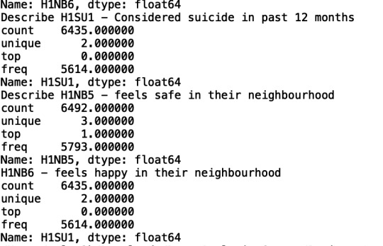
Since I do not have any quantitative variables I am unable to do a univariate analysis with a centre and spread. Instead I used the describe function for my qualitative variables to examine them further.

H1NB6 « Feels happy in their neighbourhood » has a 2 unique answers with 0 (that includes positive responses to being happy in their neighbourhood) as the most answered at a frequency of 5614. This demonstrates that almost all the respondents felt happy in their neighbourhood.

The variable H1NB5 « Feels safe in their neighbourhood » the response 1 (which includes positive responses) overshadows all other answers and demonstrates that the respondents in the sample felt almost completely safe with their neighbourhoods. The variable has has 3 unique answers, the top answer being 1 with a frequency of 5793.

The variable H1SU1 « Considered suicide in the past 12 months » has 2 unique answers with 0 (did not consider suicide) being the most answered (a frequency of 5614) demonstrating that most respondents did not consider suicide .

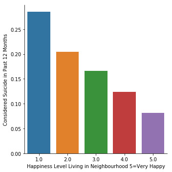
Bivariate graphs

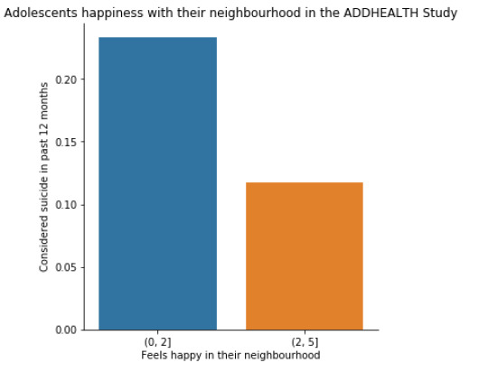
Looking at my bivariate graph I can see that respondents that feel unhappy in their neighbourhood [answers 1 and 2 (0, 2)] have a higher rate of suicide (over 0.20) in contrast with respondents that feel happy in their neighbourhood [answers 3, 4, and 5 (2, 5)] that have a rate just over (0.10). This reinforces my hypothesis that adolescents that are unhappy with their neighbourhood are more likely to consider suicide.

0 notes

stattp-blog1 · 6 years ago

Text

Making Data Management Decisions

I decided to group the values within the variable H1NB6:On the whole, how happy are you with living in your neighbourhood? I grouped answers 1 (not at all) and 2 (very little) as the negative responses and 4 (quite a bit) and 5 (very much) as the positive responses. For variable H1SU1 I coded responses 6 (refused) and 9 (not applicable)as missing and for variables H1NB5 and H1NB6 I coded responses 6 (refused) as missing as they were not relevant to answering my question.

0 notes

stattp-blog1 · 6 years ago

Text

Running Your First Program

1. Python Program

2. Frequency Tables

3. Summary

A random sample of 6,504 adolescents were asked "During the past 12 months, did you ever seriously think about committing suicide?"; of that sample, 83% chose answer 0 (no) and 12% of respondents answered 1 (yes).

When asked "Do you usually feel safe in your neighborhood?", 89% answered 1 (yes) with 10% answering 0 (no).

Moreover, respondents were asked "On the whole, how happy are you with living in your neighborhood?" 35% answered 4 (quite a bit), followed by 34% who answered 5 (very much), and 21% who answered 3 (somewhat).

0 notes

stattp-blog1 · 6 years ago

Text

Getting Your Research Project Started

My review of the AddHealth Wave questionnaire resulted in interest for studying potential correlations with suicidal thoughts. I am particularly interested in seeing if adolescents’ community environments can be associated with suicidal thinking. In my experience a person’s community environment can have a detrimental effect on a person’s mental health, specifically an adolescent’s, desire to attempt suicide. As suicidal thinking is, to me, the first step that a person experiences before attempting suicide, I chose to add to my codebook variables related to suicidal thoughts and attempts. My second topic that I chose is adolescents’ neighbourhood environment, particularly demonstrated through variables like happiness living in their neighbourhood and interactions with people in their neighbourhoods.

My research question is the following: Are suicidal thoughts in adolescents associated with their neighbourhood?

Based on my literature review, I hypothesize that adolescent’s perception of their neighbourhood (happiness living in their neighbourhood) and their social cohesion with those within it (interactions with people in their neighbourhoods) can be correlated with their mental health by form of suicidal thoughts (serious thoughts about suicide). It is in my opinion that my research using the AddHealth Wave questionnaire will validate the conclusions of Cubbin, C., LeClere, F. B., Smith, G. S., Young, R., Sweeting, H., Ellaway, A., Fagg, J., Curtis, S., Clark, C., Congdon, P., & Stansfeld, S. A. by displaying that adolescents are more likely to have suicidal thoughts if they have unhappy feelings towards living in their neighbourhoods (and vice versa).

Literature Review:

I used Google Scholar to find multiple sources on my topic using the search terms “suicide and neighbourhood” and “mental health and neighbourhood”. I found several good sources that evaluated topics directly and indirectly related to my research subject; however, I was not able to find many that I could access.

Cubbin, C., LeClere, F. B., & Smith, G. S. (2000). Socioeconomic status and injury mortality: individual and neighbourhood determinants. Journal of Epidemiology & Community Health,54(7), 517-524.

In their study, the researchers found that neighbourhood characteristics had a profound effect on suicide risks. For example, they found a 50% increased risk for suicide in people living in neighbourhoods characterized by the variables of low socioeconomic status, high racial concentration, and high residential and family instability. They suggested that such variables may increase feelings of hopelessness and social isolation in people considering suicide, which could result in an increased risk of suicide occurrences. They also found that individual socio-economic status had no effect of suicide rates which may suggest that a person’s environment (e.g. community) are a determining factor in suicide risk in individuals.

Young, R., Sweeting, H., & Ellaway, A. (2011). Do schools differ in suicide risk? The influence of school and neighbourhood on attempted suicide, suicidal ideation and self-harm among secondary school pupils. BMC public health, 11(1), 874.

Young, R., Sweeting, H., & Ellaway, A. found that suicide rates and poor mental health are higher in environments, such as neighbourhoods, where individuals’ social ties are weak, where they experience feelings of being disconnected socially, and where they feel a mismatch between their and their communities’ norms and values. They theorized that small changes in a community may have high pervasive influences on young individual’s behaviours, especially since they spend a large amount of time in their communities.

Very relevant to my research topic, the researchers explored associations of variables such as perception of local neighbourhood and suicide risk. They suggested that young peoples’ experience and perception of their local physical and social neighbourhood is related to mental health outcomes. They concluded that adolescents’ negative perceptions of the neighbourhood cohesion and safety / incivilities variables, were associated with the suicide variable. 

Fagg, J., Curtis, S., Clark, C., Congdon, P., & Stansfeld, S. A. (2008). Neighbourhood perceptions among inner-city adolescents: Relationships with their individual characteristics and with independently assessed neighbourhood conditions. Journal of Environmental Psychology, 28(2), 128-142.

This source directly compliments my research question as it investigated adolescents’ perceptions of their neighbourhoods and their mental health —as well as the conditions of their residential neighbourhood. The research specifically focused on the variables of adolescents’ feelings of attachment, alienation, satisfaction, and dissatisfaction with their area and local amenities and services, compared to variables related to individual and family attributes —most notably mental distress. They found that adolescents with higher levels of mental distress had worse perceptions of their local area.

Patterns of findings:

The patterns of findings, as a result of my literature review, are that a perosn’s neighbourhood has a determining effect on their mental health and by extension suicidal thoughts. Fagg, J., Curtis, S., Clark, C., Congdon, P., & Stansfeld, S. A. found the adolescents were the most dissatisfied with their local areas (neighbourhoods) the more they experienced mental distress. Young, R., Sweeting, H., & Ellaway, A. found that adolescent’s perceptions of their neighbourhoods were positively correlated with a suicide variable that they coded. Lastly, Cubbin, C., LeClere, F. B., & Smith, G. S. suggested that certain variables related to the condition of a person’s neighbourhood may increase feelings of hopelessness and social isolation in people considering suicide.

1 note · View note