stephininfosci

[stephininfosci]

Module 12. Assignment

Question 1

A.

B.

C.

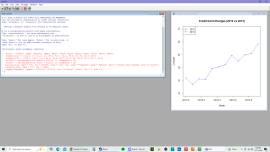
Based on the time series results, both models for 2012 and 2013 indicate that between January and December, there are upward trends. This would suggest that there is growth in spending behaviors over time when there is an increase in monthly charges.

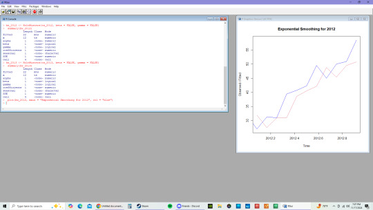
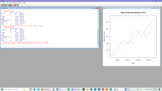
Based on the Exponential Smoothing Model, the 2012 model shows that there are short term fluctuations that are smoothed with the upward trajectory. While the 2013 model, shows a much stronger growth than the previous year as well as less fluctuations in the last half of the year in comparison to 2012.

[stephininfosci]

Module 11. Assignment

Disclaimer: I am having some difficulty with RStudio in trying to get it to run the new update, so I am just using the RGui [R Console] instead.

Question 1

With a t value of -3.2269 and a significance level of 0.005644 as well as a degree of freedom of 15, this suggests that the treatment in comparison to the placebo significantly reduces the outcome measure.

Question 2

In the model with interaction (a*b), it is more susceptible to singularities than the model with only interaction term (a:b). The fit of model (a*b) is more appropriate if the sole influence of z is from combined levels of a and b than model (a:b).

[stephininfosci]

Module 10. Assignment

Question 1

The p-values for weight, bmp, and fev1 are all less than 0.05%, while the p-value for age is greater than 0.05% before anova. This means that the weight, bmp, and fev1 are significant predictors of pemax. After anova, age, bmp, and fev1 are less than 0.05%, while weight is greater than 0.05%.

Question 2

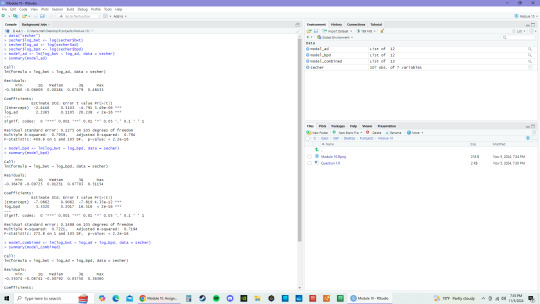
1- In the secher dataset, log-transform bwt, ad, and bpd.

2-To examine predictive strengths individually, fit individual models for bwt with ad and bpd.

3-Create a combined model with ad and bpd against bwt.

4- Interpret regression coefficients by comparing models.

With the coefficients of both log_ad and log_bpd are around 1.5, so the combined sum is about 3. This means that both have similar effects on birth weight.

When should we consider "log-transforming" a dataset? 

We should consider this when handling heteroscedasticity, when reducing outliers influence, linearizing relationships, reducing skewness, when improving model interpretability, and when data is on a multiplicative scale.

[stephininfosci]

Module 9. Assignment

Question 1

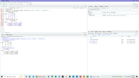
With the data given in Question 1, a one way table for "purchased" can be created by using table(df$purchased) and a one way table for "country" and "purchased" can be created using table(df$country, df$purchased).

Question 2

2.1 According to the function, there are 32 rows and 11 columns in the mtcars data set.

2.2 The proportional weight of each value in mtcars_df table are 0.03125, 0.06250, 0.37500, 0.25000, 0.12500, 0, 0.06250, 0.03125, 0.06250 as reported from using prop.table(mtcars_df).

[stephininfosci]

Module 8. Assignment

Question 1

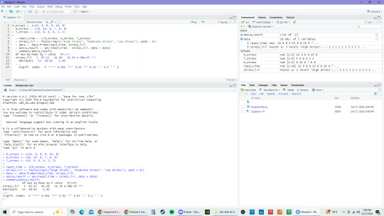
The small p value of this question's summary shows that the null hypothesis is rejected and that reaction time is linked to significant effects on stress levels.

Question 2

2.1

With half of the p values greater than 0.05 and the other half smaller than 0.05, this means that there are differences between the groups, but not in all groups.

2.2

Based on the p value of 0.129, we fail to reject the null hypothesis. This means that there does not appear to be any significant effect on reaction time based on active, passive, none, or control intervention type.

[stephininfosci]

Model 7. Assignment

Question 1

1.1 With Y as the response variable and X as the predictor variable, we can see the relationship between the two variable sets as seen in the image below. The minimum value is -11.435 and the maximum value is 16.834. The median is -4.608, while the 1st quantile is -7.406 and the 3rd quantile is 6.681.

1.2 The coefficients are 19.205597 and 3.269107.

Question 2

2.1 Waiting is the predictor variable, while discharge is the response variable.

2.2 The coefficients are -1.53317418 and 0.06755757.

2.3 The fit of eruption duration using the estimated regression equation (discharge = a + b * waiting) is predicted to be 3.871431.

Question 3

3.1 According to the data and the multiple regression model, disp, hp, and wt are all used to predict what mpg. With disp, hp and wt displaying negatives, this means that they have a negative impact on mpg. Out of all 3, it is disp that has the least negative impact on mpg, unlike hp and wt. This all means that a decrease in fuel efficiency is found when there is more horsepower and greater weight in a car.

Question 4

The predicated metabolic rate for a body weight of 70kg is about 1,305 (approximately 1,305.394).

[stephininfosci]

Module 6. Assignment

Question A

a. The mean of the entire population is 11.8.

b. The random sample of size 2 from the population were 16 and 14.

c. The mean of the sample was 15 and the standard deviation of the sample was 1.41.

d. As seen in the picture below, there is a list formed to compared the mean and standard deviation for comparison between the sample and population. The population's mean is 11.8, while the sample's mean is 15. The population's standard deviation was 3.19, while the sample's standard deviation is 1.41.

Question B

Since the sample size is n = 100 and the population proportion is p = 0.95, the distribution is expected to be normal if both np and nq are greater than 10. NP is found through 100 x 0.95, which gives us 95. NQ is found by using the equation n(1 - p) ≥ 10. (1 - 0.95) is 0.05, which means 100 x 0.05 = 5.

np ≥ 10

95 ≥ 10 (Condition is satisfied)

n(1-p)≥10 or nq≥10

5≥10 (Condition is not satisfied)

This means that the sample proportion p does not have an approximately normal distribution.

2. The smallest value of n for which the sampling distribution of p is approximately normal is found by using the equation that was previously not satisfied. Using the equation (0.05n≥10), n can be found by:

0.05n ≥ 10

n≥ 10/0.05

n=200

The smallest value of n for which the sampling distribution of p is approximately normal is n = 200.

Question C

Compared to sample(), rbinom() takes less steps than using sample () to find the outcomes, that are more efficient at the task. However, sample() requires more steps and information in it's coding to be able to complete its purpose to even be able to achieve the same outcome as rbinom().

[stephininfosci]

Module 5. Assignment

Question 1

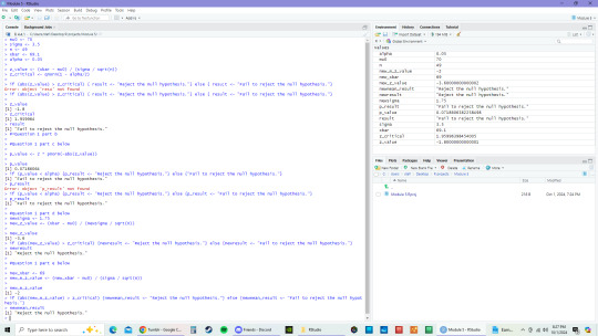
A. The null hypothesis is H0 = 70. The alternative null hypothesis is H0 =/ 70.

B. As seen in the picture below, it fails to reject the null hypothesis.

C. As seen in the picture below, the p value is 0.07186064 and it fails to reject the null hypothesis.

D. With the standard deviation changed to 1.75 for this question, new z value would be -3.6, which rejects the null hypothesis.

E. With the standard deviation changed back to the original 3.5 and the sample mean now changed to 69, the new z value would be -2 and rejects the null hypothesis.

Question 2

The 95% confidence estimate of the population mean would be (83.04, 86.96), as seen in screenshot below.

Question 3

A. The correlation coefficient for this data set is: "girls_goals" and "girls_time_spend" will likely be close to 1 and "boys_goals" and "boys_time_spend" will also likely be close to 1. This indicates that it is a positive correlation.

B. The Pearson correlation coefficient for the girls: the "girls_goals" is 1 and "girls_time_spend" is 0.9819805 (or close to 1). The Pearson correlation coefficient for the boys: "boys_goals" is 1 and "boys_time_spend" is 0.9890517 (or close to 1).

C. Plot of correlation shown in image.

Note: I, at first, had difficulty trying to get corrgram() to work on my coding without an error code popping up. I was confused as to what I was missing and the packages in the box in the lower right hand corner were not showing corrgram. To solve this, I found that typing install.packages("corrgram") was able to resolve my issue since I did not have this packaged installed before.

[stephininfosci]

Module 4. Assignment

For Part A of the assignment, the task was to find the probability of event A, event B, event A or B, and finally, finding P(A or B) = P(A) + P (B). For my results (see picture below), I have found that the probability of event A/ event B happening is 0.333333. The likely of A or B happening is 0.555555. The likely of A and B happening is 0.111111.

For Part B of the assignment, the task is to determine on whether or not the probability of the 11% chance of rain is true or false on Jane's wedding day in the desert and then to explain why. After using the Bayes' Theorem, the answer given is 0.1111111111, which if multiplied by 100 would give us 11.1%. This means that the 11% chance of it raining on Jane's wedding day is true. According to the data given, it has only rained 5 days out of the whole year in this desert region, so it is very rare to have rain and the probability remains low, despite the weatherman's predictions.

Note: please pardon the errors in the console of the image below, I was trying to display the answer.

For Part C of the assignment, the task was to find the probability of operating on 10 patients successfully with a postoperative complication frequency of 20% and the surgeon has operated on 10 patients with no complications. By using the function dbinom in R, I found that the probability of operating on 10 patients successfully is 0.1073742 or about 10.7%.

[stephininfosci]

Module 3. Assignment

In this assignment, I used 2 data sets to find it's mean, medium, and mode under Central Tendency. As well as both sets' range, interquartile, variance, and standard deviation under Variation. The screenshots below show my coding in the console and the descriptive writing of the code.

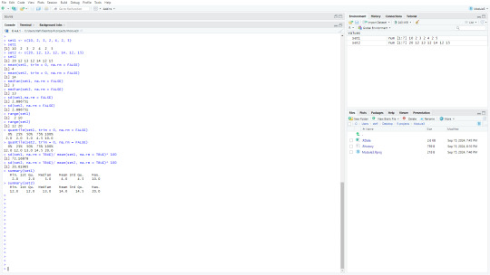
In set1 (10, 2, 3, 2, 4, 2, 5) and set2 (20, 12, 13, 12, 14, 12, 15), there are clear similarities and differences with this data. Like how set2 is just set1, but with 10 added to each number. The standard deviation for each set even turns out to be the same answer, 2.886751. And if you were to calculate the difference of the range, both sets would come up with the number 8.

While there are similarities, there are also a lot of differences between these sets. With set1's numbers being smaller than set2's, the output for set1's mean, median, range, interquartile, and summary are smaller than set2's output. However, it is opposite in regards to coefficient of variation, where the smaller set receives a larger number than the larger set.

[stephininfosci]

Module 2- R assignment2

In this assignment, the instructions were to find the mean of the given dataset {6, 18, 14, 22, 27, 17, 22, 20, 22}. The function "assignment2" holds this dataset that will be calculated by myMean. The results came out to 18.66667.

While working on this assignment, I wanted to see what would happen if the function(x) remained x instead of placing in assignment2. I have highlighted the line that was changed. This was the result:

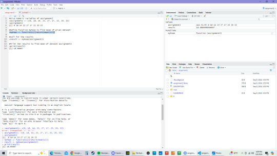
Though the results are the same in both, it is important to define the function because if this was a bigger dataset instead of just this one isolated one, there is a chance that the data would mess up somewhere along the way with other datasets.