#Compute the sum of the first 5 values

[balancetarot]

should I write about sigils and kameas and magic squares?

because I've been slightly obssessed with the topic lately, and frankly it's fascinating. or maybe I'm a huge nerd that thinks fun with math is a good time. esoteric math!

...fuck it. I'm gonna do it.

so a magic square is a fun thing that happens in math where you have a table with an equal number of rows and columns, and in that table each row, column, and corner to corner diagonal, adds up to the same sum. that sum is called the 'magic constant'. the number of rows/columns is the Order of the square.

some squares are extra fancy, and may have other subsets that add to the same sum; say a four by four square in which every subset of four squares adds to the same sum. (check out the Chautisa Yantra, it's great.)

our ancestors looked at this sort of fun with math and thought something like "this is so neat, it must be meaningful." or maybe that it's such an interesting pattern it must be derived from a higher power. and thus, magic.

each magic square has a minimum value for its magic constant, and if you try to build a square with a lower constant, you have to use fractions instead of whole numbers, or even negative numbers.

when folks get started messing with making talismans, for some reason, they start with the Saturn square. I get it, it's easy. the Saturn square has three rows and three colums, uses all numbers 1 through 9, and has a constant value of 15. it's cute, and simple, and graphing out your sigil on it is easy.

see? that's the Saturn Square. Order 3, Constant 15 (and if you add up all the digits, it adds up to 45).

but that's just getting started!

by the time of the writing of the Picatrix, and Agrippa's Three Books of Occult Philosophy (1500's) magic squares up to Order 9 were known, and had been assigned to planetary and luminary bodies. (luminaries are the sun and moon.)

because the modern planets cannot be seen without a telescope, Uranus, Neptune, and Pluto (a planet in my heart!) don't have magic squares assigned to them.

with the rise of machine computing, we have found higher order magic squares, including up to Order 260 or more. which is good, because the idea of doing that much math makes me kinda want to whimper.

Jupiter, Order 4, constant 34

Mars, Order 5, Constant 65

Sun, Order 6, Constant 111

Venus, Order 7, Constant 175

Mercury, Order 8, Constant 260

Moon, Order 9, Constant 369

while most instructions for making a sigil will tell you to assign a number value to your letters, add 'em up, and keep adding until you get a single digit, that's really only super useful for the Saturn square, where none of the digits in it are higher than 9.

if you're using a different square, you don't have to reduce your numbers to single digits, though you do need to be aware of what the upper limit for the value of individual points in your square are. how do you figure that out? take your Order and square it.

an Order 4 square has an upper value of 16. an Order 7 square tops out at 49. and so on!

*~*~*~*~*~*~*~*~*~*~*~*~*~*~*~*~*~*~*~*

I'm currently experimenting to attempt to figure out what higher order squares should be associated with Uranus and Neptune (Pluto's not a priority right at this moment for me, I figure it'll be obvious once I assign those first two.)

you've doubtless noticed that all the squares from 3 to 9 have been assigned to something, without skipping one and leaving it unassigned! logically, this means Order 10, 11, and 12 squares can be assigned to Uranus, Neptune, and Pluto. the problem is: those lower order squares aren't assigned to the planets in order. so we can't just say "oh, Order 10 goes with Uranus, cause it's next in line".

want to join me in experimentation? here's an Order 10 square, constant 505:

might be Uranus, Neptune, or Pluto. dunno!

it's clearly time to FA and FO.

(yes, I've spent the last week pickling my brains with magic squares. you're welcome.)

[blake447]

Arcane method of drawing the Von Koch Curve

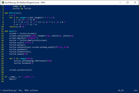
So, some of you might remember my old post about the dragon curve, and an odd way of drawing that by calculating the nth term as a sum of bits in series of binary sequences. For those that haven't seen it, go check that out, its more understandable I think. Also, note that while this is using turtle graphics, we use absolute heading rather than angles left or right. This means that each term is entirely independent and could be calculated in parallel using multi-threading or even a GPU if for some reason you wanted to.

But Blake, I hear you asking, how do you express the Von Koch curve as a sum of bits in a series of binary sequences. Well, I'm glad you asked! Well, we start by once again assigning modular integers to each of the possible directions required to draw the curve, modular simply meaning that once we go above a certain number (5) we simply rollover back to zero. We call this (mod 6). Once we do that, we examine how we can boil the curve down into a sequence using these numbers. By inspection, we see one interpretation being to start with 0, expand the sequence by a factor of 4, and strike the middle two quartiles out, adding one to the first inner quartile, and subtracting one from the second inner quartile, as shown in the process below

And again as with the dragon curve, we can rearrange the order we do this and propagate the added and subtracted ones, which when following the expansion by a factor of four forms alternating patterns. Now from some information theory, since we have positive and negative ones to represent, we need two bits in order to represent the each term in the series, hence the two bit sequences.

Unlike last time, I've actually formalized this a little bit. Here is the derivation for the rules on generating arbitrary sequences of power of two times repeating 0's and 1's, with the ability to offset the start of the sequence, as was necessary with the dragon curve.

Now we can take that formalization, do a bit of inspection of the sequences necessary to compose the adding / subtracting pattern, and derive a series formula that calculates the nth term of this manner of representing the Von Koch curve

Finally, now that we have our series representation, we can modify our original dragon curve code and generate a Von Koch curve after we've translated the series into computer instructions. Note that powers of 2 turn into bit shifts of 1, and indexing requires bit shifting the value and bitwise and-ing with 1 to get the desired bit, calculate the length of the sequence on the back of an envelope aaaaaand....

Holy shit it just worked?... I mean voila! It uh, it draws a koch curve. With the bonus that this code is entirely un-fucking-readable unless you're insane, like me. But yeah, really having fun with this binary sequence stuff because its cool as hell.

[acorgiirl]

Project Euler #2

Welcome back to my series on Project Euler problems. HackerRank Lets get into it.

Links:

Project Euler: https://projecteuler.net/problem=2 HackerRank: https://www.hackerrank.com/contests/projecteuler/challenges/euler002

Each new term in the Fibonacci sequence is generated by adding the previous two terms. By starting with 1 and 2, the first 10 terms will be: 1,2,3,5,8,13,21,34,55,89,… By considering the terms in the Fibonacci sequence whose values do not exceed N, find the sum of the even-valued terms.

So first thing to note is just how odds and evens work. This starts with 1 and 2 so Odd + Even = Odd, then the next term would just be Even + Odd = Odd. It isn't until the 3rd addition that we get Odd + Odd = Even. After that this cycle will repeat.

So really what this is asking for is, starting at index 2, what is the sum of every 3rd term less than N.

F(2) + F(5) + ... + F(3k + 2)

(Where F(N) is the Nth Fibonacci number)

Now, computing Fibonacci numbers notoriously sucks to do, with the naive way of doing it causing you to compute from just F(20) would require computing F(3) like hundreds if not thousands of times over. So the best way to do it is to create either a hash or a cache to store it. I'm going to be utilizing something built into Python, "lru_cache" from the "functools" module. It'll just store the answers for me so I don't have to recompute what F(10) is thousands of times.

Here's my HackerRank code:

import sys from functools import lru_cache @lru_cache def fibonacci(N: int) -> int: if N < 0: return 0 if N <= 1: return 1 return fibonacci(N-1) + fibonacci(N-2) t = int(input().strip()) for a0 in range(t): n = int(input().strip()) x = 2 f = fibonacci(x) total = 0 while f <= n: total += f x += 3 f = fibonacci(x) print(total)

So as you can see, I just start at 2 and keep incrementing by fibonacci number by 3 each time. Then the loop will stop when my fibonacci number exceeds N.

And that's all tests passed! Onto the next one!

[lucajack123]

How to Learn Power BI: A Step-by-Step Guide

Power BI is a powerful business intelligence tool that allows users to analyze data and create interactive reports. Whether you’re a beginner or looking to enhance your skills, learning Power BI can open doors to career opportunities in data analytics and business intelligence. For those looking to enhance their skills, Power BI Online Training & Placement programs offer comprehensive education and job placement assistance, making it easier to master this tool and advance your career.

Here’s a step-by-step guide to mastering Power BI.

Step 1: Understand What Power BI Is

Power BI is a Microsoft tool designed for data analysis and visualization. It consists of three main components:

Power BI Desktop – Used for building reports and dashboards.

Power BI Service – A cloud-based platform for sharing and collaborating on reports.

Power BI Mobile – Allows users to access reports on smartphones and tablets.

Familiarizing yourself with these components will give you a clear understanding of Power BI’s capabilities.

Step 2: Install Power BI Desktop

Power BI Desktop is free to download from the Microsoft website. It’s the primary tool used to create reports and dashboards. Installing it on your computer is the first step to hands-on learning.

Step 3: Learn the Power BI Interface

Once installed, explore the Power BI interface, including:

Home Ribbon – Where you access basic tools like importing data and formatting visuals.

Data Pane – Displays the data tables and fields available for reporting.

Visualizations Pane – Contains different chart types, tables, and custom visuals.

Report Canvas – The workspace where you design and organize your reports.

Getting comfortable with the interface will make learning easier.

Step 4: Import and Transform Data

Power BI allows you to connect to various data sources like Excel, SQL databases, and cloud applications. Learning how to:

Import data from multiple sources.

Use Power Query Editor to clean and shape data.

Handle missing values, remove duplicates, and structure data for analysis. It’s simpler to master this tool and progress your profession with the help of Best Online Training & Placement programs, which provide thorough instruction and job placement support to anyone seeking to improve their talents.

Data transformation is a crucial step in building accurate and meaningful reports.

Step 5: Create Visualizations

Power BI provides multiple visualization options, including:

Bar charts, pie charts, and line graphs.

Tables, matrices, and cards.

Maps and custom visuals from the Power BI marketplace.

Experimenting with different visualizations helps you present data effectively.

Step 6: Learn DAX (Data Analysis Expressions)

DAX is a formula language used in Power BI to create calculated columns, measures, and custom calculations. Some key DAX functions include:

SUM() – Adds values in a column.

AVERAGE() – Calculates the average of a set of values.

IF() – Creates conditional calculations.

Mastering DAX enables you to perform advanced data analysis.

Step 7: Build and Publish Reports

Once you’ve created a report, learn how to:

Organize multiple pages in a dashboard.

Add filters and slicers for interactive analysis.

Publish reports to Power BI Service for sharing and collaboration.

Publishing reports makes them accessible to teams and decision-makers.

Step 8: Explore Power BI Service and Cloud Features

Power BI Service allows you to:

Schedule automatic data refreshes.

Share dashboards with team members.

Implement row-level security for restricted data access.

Learning cloud-based features enhances collaboration and security in Power BI.

Step 9: Join Power BI Communities

Engaging with the Power BI community can help you stay updated with new features and best practices. You can:

Follow the Microsoft Power BI blog for updates.

Participate in Power BI forums and LinkedIn groups.

Attend webinars and join Power BI user groups.

Networking with other Power BI users can provide valuable insights and learning opportunities.

Step 10: Get Certified and Keep Practicing

If you want to showcase your expertise, consider obtaining a Microsoft Power BI Certification (PL-300: Power BI Data Analyst). Certification enhances your resume and validates your skills.

To stay ahead, keep practicing by working on real-world datasets, building dashboards, and experimenting with advanced Power BI features. Continuous learning is the key to becoming a Power BI expert.

By following these steps, you can systematically learn Power BI and develop the skills needed to analyze and visualize data effectively. Happy learning!

[strattonxpressions]

Ethan Lee

1. Name, Year, Major, and Hometown

Ethan Lee, Third Year Computer Science Major, San Mateo CA

2. What is your earliest childhood memory? 

My earliest childhood memory is going to Chinatown for egg tarts and dim sum in preschool with my parents and grandparents.

3. What’s stopping you?

The one thing that is stopping me is time.

4. What is something about yourself that you’re proud of?

Something about myself that I am proud of is not getting a parking ticket yet.

5. If you could have any one question answered truthfully, what would it be?

What are the powerball lottery numbers for next week?

6. Who is your celebrity/fictional crush? 

My celebrity crush is Saerom from fromis_9.

7. How would you spend your ideal birthday? 

I would ideally spend my birthday exploring a destination I have never been before such as Singapore, New York or Tokyo.

8. What food that starts with the first letter of your name would you only eat for the rest of your life?

One food that starts with the letter E and would eat for the rest of my life is egg tarts.

9. What’s one niche interest you have that you must share with the world?

like wasting time by looking at stocks and google flights.

10. What is a memory with your closest friend and how does it exemplify your friendship together and how you value friendship as a whole (250 words minimum)

During the end of senior year, I supported one of my friends who struggled during the college admissions process and helped her navigate alternative options when she dealt with unexpected admissions decisions. To many, she would be considered an outstanding student with good grades, heavy extracurricular and community involvement, and high scores in the SAT and AP exams. In particular, she was known to be an exceptional writer, often scoring the highest in the class on essays, research papers, and timed writes. She had future career aspirations in law and wanted to pursue a career in corporate law. To everyone’s surprise, she was rejected from every college she applied to except for the University of Wisconsin, where she was waitlisted. Devastated by her decisions, she had difficulty determining what her options were. Although she faced pressure from her family and other figures to attend the University of Wisconsin because it was the only college that accepted her, she had several hesitations including out-of-state tuition, the weather, overall campus culture, and location in the Midwest. Alternatively, her dream school was UC Santa Barbara, and her other option was attending community college and transferring to UCSB. Although some of our mutual friends believed she would have been successful attending UW Madison, the conversations I had with her about what she wanted in college and what she planned to do convinced her to attend community college. Two years later, she is a political science and sociology double major at UCSB and is currently preparing for the LSAT. She agrees that attending community college and transferring was the better option and allowed her to become more prepared and eager to pursue a career in law. Ultimately, this experience allowed me to recognize the importance of friendship and how unique each specific relationship is. Everyone has their own path in life and as a friend, I should do what's necessary to help them pursue their goals rather than having them conform to a specific expectation.

[tccicomputercoaching]

5 JavaScript functions every developer should know

"JavaScript developers! In this learning today, we will look at 5 functions that will get you to the next level of coding. Let's get started!"

"The first is map(). This is used to change every element of an array. If it just wants to double numbers, then it's great.”

"The second is filter(). Used to filter out a specific element of a array. for instance, to only delete the even numbers.”

"The third is reduce(). “It takes an array of elements and brings it all together to return a single value: the totalized sum or product.”

"The fourth is find(). It finds the first element in the array that satisfies a given condition. As an example, the first even number.

"The last is forEach(). It is basically used when you want to do something to each element of an array.”

TCCI Tririd Computer Coaching Institute offers web design course in Bopal and Iskon-Ambli road in Ahmadabad.

Web Design Course includes HTML, CSS, Java Script, Image Making, Boot strap etc.

You can join full course or learn any one language of the course.

TCCI provide online coaching to any person, any place.

For More Information:

Call us @ +91 98256 18292

Read more @ https://tccicomputercoaching.wordpress.com/

[ensafomer]

 Testing a Potential Moderator

Research: Testing for a Potential Mediator Using ANOVA

Introduction: Testing for a potential mediator is a statistical method used to examine if a third variable (mediator) affects the relationship between two other variables. This mediator can contribute to understanding the mechanism by which the independent variable influences the dependent variable. By identifying the mediator, researchers can gain deeper insights into the causal processes underlying the relationship.

In this study, we will use Analysis of Variance (ANOVA) to test for the potential mediating effect of physical activity on the relationship between treatment type and disease outcome.

1. Objectives:

Research Objective: Analyze the relationship between treatment type (independent variable) and disease outcome (dependent variable) using ANOVA, and test for physical activity as a mediator.

Research Questions:

Does physical activity affect the relationship between treatment type and disease outcome?

Can physical activity be considered a mediator in this relationship?

2. Variables:

Independent Variable: Treatment type (e.g., medication treatment vs. physical therapy treatment).

Dependent Variable: Disease outcome (e.g., improvement in health).

Mediator Variable: Physical activity level.

3. Hypotheses:

Null Hypothesis (H0): There is no effect of physical activity on the relationship between treatment type and disease outcome.

Alternative Hypothesis (H1): There is an effect of physical activity on the relationship between treatment type and disease outcome.

4. Methodology:

In this study, we will use ANOVA to test whether physical activity mediates the relationship between treatment type and disease outcome.

Steps for Analysis:

Data Collection: The dataset contains information on treatment type, physical activity level, and disease outcome. The data will be in a table format with the following columns:

Outcome: Disease outcome (degree of improvement or deterioration).

Treatment: Treatment type (e.g., medication, physical therapy).

PhysicalActivity: Physical activity level (e.g., low, moderate, high).

Statistical Analysis: We will use ANOVA to test for the interaction between Treatment and PhysicalActivity on the Outcome.

Hypothesis Testing: Using statistical values such as F-statistic and p-value, we will determine whether the interaction is statistically significant.

5. Software Tools Used:

We will use Python programming language and its statistical libraries for data analysis, particularly:

pandas for data manipulation.

statsmodels for performing ANOVA.

6. Implementing ANOVA in Python:

Code Example:

Explanation of the Code:

First, we load the data from a CSV file using pandas.

Then, we use the ols() function from the statsmodels library to create an ANOVA model that includes the interaction between Treatment and PhysicalActivity on Outcome.

Finally, we use sm.stats.anova_lm() to compute the results of the ANOVA and display the output in a table.

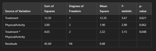
7. Results:

After performing the analysis, we will obtain an ANOVA table with the following components:

Sum of Squares: This shows the variance explained by each factor (Treatment, PhysicalActivity, and their interaction).

Mean Square: This is calculated by dividing the Sum of Squares by the degrees of freedom (Degrees of Freedom).

F-statistic: This measures how much the factors influence the outcome.

p-value: The p-value indicates whether the interaction is statistically significant.

Assuming the results are as follows (for illustrative purposes):

8. Interpretation:

Interaction between Treatment and Physical Activity: Since the p-value for the interaction term (Treatment * PhysicalActivity) is 0.048 (less than 0.05), we reject the null hypothesis and conclude that there is a statistically significant interaction between treatment type and physical activity affecting the disease outcome.

Effect of Physical Activity: The p-value for physical activity alone is 0.062, which is greater than 0.05, indicating that physical activity alone does not have a statistically significant effect on the disease outcome in this case.

Effect of Treatment: The p-value for treatment is 0.021, which is less than 0.05, indicating that treatment type has a statistically significant effect on the disease outcome.

9. Conclusion:

From the results of the ANOVA analysis, we conclude that physical activity acts as a mediator between treatment type and disease outcome. The interaction between treatment and physical activity was statistically significant, suggesting that physical activity influences the way treatment affects the disease outcome.

10. Future Recommendations:

Larger sample size: Using a larger sample could provide more accurate and reliable results.

Comparative studies: Comparing the effects of other factors on treatment and outcome could help provide a more comprehensive understanding.

Testing other mediators: Exploring other potential mediators, such as nutrition or psychological factors, might reveal additional insights into the treatment-outcome relationship.

Conclusion:

Using ANOVA to test for potential mediators provides an effective means of understanding the relationship between variables and how mediating factors influence these relationships. In this research, we found that physical activity acts as a mediator between treatment type and disease outcome, opening avenues for further studies that could apply these findings to improve healthcare treatments.

[krishnaacademyrewa]

Master 10 Basic Excel & Google Sheets Formulas in One Class! Enhance Your Spreadsheet skills!

Unlock the power of Excel and Google Sheets with Krishna Academy Rewa! In this class, we'll cover 10 essential formulas and functions that will help you master spreadsheet tasks with ease. Visit More : https://www.youtube.com/watch?v=TQb35cjMFzw

What You'll Learn:

1. SUM: Add up a range of numbers effortlessly.

2. COUNTA: Count the number of non-empty cells.

3. MAX & MIN: Find the highest and lowest values in your data.

4. AVERAGE: Calculate the mean value.

5. CONCATENATE: Combine text from multiple cells.

6. COUNT: Count the number of cells that contain numbers.

7. UPPER & LOWER: Convert text to uppercase or lowercase.

8. PROPER: Capitalize the first letter of each word. Why Join Us?

1. Expert Instruction: Learn from experienced professionals at Krishna Academy Rewa.

2. Hands-On Learning: Practical examples and exercises to help you understand and apply each function.

3. Versatile Skills: These formulas are crucial for various tasks in both Excel and Google Sheets.

Don't miss this opportunity to enhance your spreadsheet skills! Subscribe to our channel for more tutorials and visit Krishna Academy Rewa for advanced courses on computer applications. -

- - #excelformulas - #GoogleSheetsFormulas - #spreadsheettips - #exceltutorial - #googlesheetstutorial - #BasicExcelFunctions - #BasicGoogleSheetsFunctions - #KrishnaAcademyRewa - #excelforbeginners - #GoogleSheetsForBeginners - #learnexcel - #LearnGoogleSheets - #computereducation - #onlinelearning - #dataanalysis - #SpreadsheetTraining - #exceltips - #googlesheetstips

[juliebowie]

Introduction to Armstrong Number in Python

Summary: Discover the concept of Armstrong Numbers in Python, their unique properties, and how to implement a program to check them. Learn about basic and optimised approaches for efficient computation.

Introduction

In this article, we explore the concept of an Armstrong Number in Python. An Armstrong number, also known as a narcissistic number, is a number that equals the sum of its own digits, each raised to the power of the number of digits. 

These numbers are significant in both programming and mathematical calculations for understanding number properties and algorithmic efficiency. Our objective is to explain what an Armstrong number is and demonstrate how to implement a program to check for Armstrong numbers using Python, providing clear examples and practical insights.

Read: Explaining Jupyter Notebook in Python.

What is an Armstrong Number?

An Armstrong number, also known as a narcissistic number, is a particular type of number in which the sum of its digits, each raised to the power of the number of digits, equals the number itself. This property makes Armstrong numbers unique and exciting in mathematics and programming.

Definition of an Armstrong Number

An Armstrong number is defined as a number equal to the sum of its digits; each raised to the power of the total number of digits. For example, if a number has 𝑛 digits, each digit d is raised to the 𝑛th power and the sum of these values results in the original number.

Explanation with a Simple Example

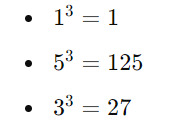
Consider the number 153. It has three digits, so we raise each digit to the third power and sum them:

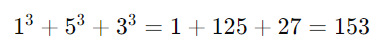
Since the result equals the original number, 153 is an Armstrong number. Another example is 370:

Difference Between Armstrong Numbers and Other Numerical Concepts

Armstrong numbers are distinct because they involve the specific property of digit manipulation. Unlike prime numbers, which are based on divisibility, or perfect numbers, which relate to the sum of divisors, Armstrong numbers focus solely on digit power sums. This unique characteristic sets them apart from other numerical concepts in mathematics.

How to Determine an Armstrong Number?

To determine whether a number is an Armstrong number, we need to verify if the sum of its digits, each raised to the power of the number of digits, equals the number itself. This concept may seem complex at first, but with a clear understanding of the process, it becomes straightforward. 

Let's break down the steps and explore the mathematical method used to identify Armstrong numbers.

Mathematical Formula

The formula to check if a number is an Armstrong number is: 

Here, d1,d2,…,dm​ represent the digits of the number, and 𝑛 is the total number of digits.

Step-by-Step Breakdown

Determine the Number of Digits: First, find the total number of digits, nnn, in the given number. This is crucial as each digit will be raised to the power of nnn.

Extract Each Digit: Extract each digit of the number. This can be done using mathematical operations like modulus and division.

Raise Each Digit to the Power of nnn: For each digit, calculate its power by raising it to nnn.

Sum the Powered Digits: Add the results of the previous step together to get the sum.

Compare the Sum with the Original Number: Finally, compare the sum with the original number. If they are equal, the number is an Armstrong number.

Example Calculation

Let's determine if 153 is an Armstrong number:

Number of digits (n): 3

Extracted digits: 1, 5, 3

Raised to the power of n:

Sum of powered digits: 1+125+27=1531

Comparison: The sum, 153, equals the original number, confirming that 153 is an Armstrong number.

This systematic approach helps in accurately identifying Armstrong numbers, making the concept both interesting and accessible.

Also Check: Data Abstraction and Encapsulation in Python Explained.

Armstrong Number Algorithm

An Armstrong number, also known as a narcissistic number, is a number that is equal to the sum of its own digits each raised to the power of the number of digits. To determine if a number is an Armstrong number, we follow a specific algorithm. 

This section outlines the steps involved and discusses the efficiency and complexity of the algorithm.

Outline of the Algorithm

To check if a number is an Armstrong number, follow these steps:

Determine the Number of Digits:

First, calculate the number of digits (n) in the given number. This step helps in raising each digit to the appropriate power.

Calculate the Sum of Digits Raised to the Power of n:

For each digit in the number, raise it to the power of n and sum these values. This step involves iterating through each digit, performing the power operation, and accumulating the results.

Compare the Sum with the Original Number:

Finally, compare the calculated sum with the original number. If they are equal, the number is an Armstrong number.

Key Steps in the Algorithm

Extracting Digits: We extract each digit from the number, which can be done using modulus and division operations.

Power Calculation: Raise each extracted digit to the power of the total number of digits.

Summation: Accumulate the results of the power calculations to form the total sum.

Comparison: Compare the accumulated sum with the original number to determine if it is an Armstrong number.

Efficiency and Complexity

The Armstrong number algorithm is efficient for small to moderately sized numbers. The primary operations involve basic arithmetic, such as modulus, division, and exponentiation, making the algorithm computationally light. The time complexity is O(d), where d is the number of digits in the number. 

This is because the algorithm processes each digit exactly once. For large numbers, the time complexity may increase, but it remains manageable due to the simplicity of the calculations involved.

Implementing Armstrong Number in Python

To determine whether a number is an Armstrong number, we need to implement a straightforward approach in Python. Armstrong numbers, also known as narcissistic numbers, are numbers that equal the sum of their own digits each raised to the power of the number of digits. 

Here, we’ll explore a basic implementation in Python and discuss how to optimise it for better performance.

Basic Implementation

Let’s start with a simple Python program to check if a number is an Armstrong number:

Explanation of the Code:

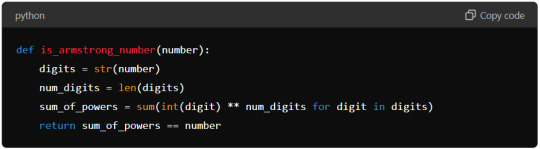
Function Definition: The function is_armstrong_number takes an integer number as its parameter.

Convert Number to String: We convert the number to a string using str(number) to easily access each digit.

Count Digits: We determine the number of digits using len(digits).

Initialise Sum Variable: We initialise sum_of_powers to zero to accumulate the sum of each digit raised to the power of num_digits.

Calculate Sum of Powers: We loop through each digit in the string, convert it back to an integer, raise it to the power of num_digits, and add it to sum_of_powers.

Check Armstrong Condition: Finally, we compare sum_of_powers with the original number to determine if it is an Armstrong number.

Optimised Approach

While the basic implementation is easy to understand, it may not be the most efficient for larger numbers. Here are some optimisations:

Use List Comprehension: Python’s list comprehension can make the code more concise. Here’s an optimised version:

This version uses a single line to calculate sum_of_powers using list comprehension, making the code more compact and potentially faster.

2. Precompute Powers: For very large numbers, precomputing powers for digits (0 through 9) and reusing them can reduce computation time.

3. Avoid String Conversion: If working with extremely large numbers, you might want to avoid converting numbers to strings repeatedly. However, this is a trade-off between readability and performance.

By employing these optimisations, you can enhance the efficiency of the Armstrong number checking algorithm, especially for larger inputs.

Frequently Asked Questions

What is an Armstrong Number in Python?

An Armstrong Number in Python is a number that equals the sum of its digits each raised to the power of the number of digits. For example, 153 is an Armstrong Number because 1^3+5^3+3^3=153.

How can I check for an Armstrong Number in Python?

To check for an Armstrong Number in Python, calculate the sum of each digit raised to the power of the total number of digits. If this sum equals the original number, it’s an Armstrong Number.

What is the efficiency of the Armstrong Number algorithm in Python?

The Armstrong Number algorithm in Python is efficient for small to moderate numbers with a time complexity of O(d), where d is the number of digits. The primary operations include basic arithmetic and exponentiation.

Further See: Understanding NumPy Library in Python.

Conclusion

In this article, we've explored Armstrong Numbers in Python, highlighting their unique property of being equal to the sum of their digits raised to their respective powers. We demonstrated how to implement and optimise a Python program to check for Armstrong Numbers. Understanding this concept and its implementation enhances both mathematical knowledge and programming skills.

[workforcesolution]

R AND PYTHON GRADIENT DESCENT

My previous blog, I presented syntactical differences and similar functions between R & Python. Now, I want to take it to next level and write some machine learning algorithms using both R and Python. Here, one may use direct functions from the packages available. However, here I am presenting the way to write your own functions for algorithms. In this series, I am starting with Gradient descent algorithm. I briefly explain, what is gradient descent. After that, I apply gradient descent algorithm for a linear regression to identify parameters. For illustration, I simulate data for simple linear regression. I show how you can write your own functions for simple linear regression using gradient descent in both R and Python. I present the results of both R and Python codes.

Gradient descent algorithm

Gradient descent is one of the popular optimization algorithms. We use it to minimize the first order derivative of the cost function. You can define a cost function using an equation (example: f(x) = 3x2 + 2x+3) , then do the first order derivative for it ( in this case, f `(x)= 6x+2). Then you can randomly initialize value of x and iterate the value with some learning rate (slope), until we reach convergence (we reach local minimum point). For more details, you can refer simple computational example, with python code, given in Wikipedia . I am taking the same concept of Gradient Descent and applying it for simple linear regression. In the above example, we have the equation to represent the line and we are finding the minimum value. However, in the case of linear regression, we have data points, and we come up with the linear equation, that fits these data points. Here, it works by efficiently searching the parameter space to identify optimal parameters i.e,or . intercept(theta0) and slope(theta1). We initialize the algorithm with some theta values and iterate the algorithm to update theta values simultaneously until we reach convergence. These final theta values (parameters or coefficients), when we put it in equation format, represent best regression line. In machine learning, the regression function y = theta0 + theta1x is referred to as a 'hypothesis' function. The idea, just like in Least squares method, here is to minimize the sum of squared errors, represented as a 'cost function'. We minimize cost function to achieve the best regression line. Let us start with simulating data for simple linear regression.

R:

Importing the dummy data we created. setwd("S:\\ANALYTICS\\R_Programming\\Gradient_Descent") N x beta errors # errors errors y data colnames(data) write.csv(data, file = "Data.csv", row.names = FALSE) Below we are considering the above simulated data for the python coding purpose. #Data simulation for python colnames(data) write.csv(data, file = "Data_Python.csv", row.names = FALSE) Looking at the dimension of data this is because we are working on matrix method. Now we change the dimension of x(predictor) and y(response) accordingly to make matrix multiplication possible. create the x- matrix of explanatory variables. Here we are producing a matrix with 1's in 100 rows to make the matrix dimension is such a way that the multiplication is possible. Data head(Data) ## x y ## 1 55.01790 26.34163 ## 2 63.62490 36.61669 ## 3 56.07122 26.69499 ## 4 61.00054 39.82381 ## 5 63.45294 36.48111 ## 6 62.82037 32.28978 dim(Data) ## [1] 100 2 head(Data) ## x y ## 1 55.01790 26.34163 ## 2 63.62490 36.61669 ## 3 56.07122 26.69499 ## 4 61.00054 39.82381 ## 5 63.45294 36.48111 ## 6 62.82037 32.28978 attach(Data) #n a0 = rep(1,100) a1 = Data[,1] b = Data[,2] x y head(x) ## a0 a1 ## [1,] 1 55.01790 ## [2,] 1 63.62490 ## [3,] 1 56.07122 ## [4,] 1 61.00054 ## [5,] 1 63.45294 ## [6,] 1 62.82037 head(y) ## [,1] ## [1,] 26.34163 ## [2,] 36.61669 ## [3,] 26.69499 ## [4,] 39.82381 ## [5,] 36.48111 ## [6,] 32.28978

Derivative Gradient:

Derivative gradient is the next step after simulating the data in which we obtain the initial parameters. For initializing the parameter of hypothesis function, we considered the first order derivative of the cost function in the below function. where m is the total number of training examples and h(x(i)) is the hypothesis function defined like this: Hypothesis Equation For determining the initial gradient values, we have to consider the first derivative of the cost function which shown below. Cost function J(theta0, theta1) Cost Function Initial_Gradient m hypothesis = x %*% t(theta) loss = hypothesis - y x_transpose = t(x) gradient return(t(gradient)) } Here 'i' represents each observation from the data. For the derivative gradient, we are determining the first derivative of the cost function which gives initial coefficients to update through the gradient runner below. This derivative gradient is called by the gradient runner inside the for loop. From the above function results we will get the matrix of thetas (a0 and a1). Now using the gradient runner, we have to iterate through the theta0 and theta1 until convergence.

Gradient runner:

Gradient runner is the iterative process to update the theta values through the below function until it converges to its local minimum of the cost function. Here in this function additional element we are using is learning rate(alpha) which help to converge to local minimum. For our requirement, we considered alpha as 0.0001. Gradient descent is used to minimize the cost function to get the converged theta value matrix which fits the regression line in data. gradient_descent # Initialize the coefficients as matrix theta #theta #learning rate alpha = 0.0001 for (i in 1:Numiterrations) { theta } return(theta) } print(gradient_descent(x, y, 1000)) ## a0 a1 ## [1,] 0.03548202 0.5777683 To speed up the convergence change learning rate or number of iterations. If you consider learning rate as too small it will take more time to converge and if it is high also it will never converge.

Python:

Import all the required packages and the dummy data to run the algorithm. For python, also we are doing it in matrix method. Same steps to be followed in python as we did using R. from numpy import * import numpy as np import random from sklearn.datasets.samples_generator import make_regression import pylab from scipy import stats import pandas as pd import os path = "S:\\ANALYTICS\\R_Programming\\Gradient_Descent" os.chdir(path) points = genfromtxt("Data_Python.csv", delimiter=",", ) a= points[:,0] b= points[:,1] x= np.reshape(a,(len(a),1)) x = np.c_[ np.ones(len(a)), x] # insert column y = b #For determining the initial gradient values, we have to consider the first derivative of the cost function which shown below. Cost function def Initial_Gradient(x, y, theta): m = x.shape[0] hypothesis = np.dot(x, theta) loss = hypothesis - y x_transpose = x.transpose() gradient = (1/m) * np.dot(x_transpose, loss) return(gradient) #Below gradient descent function is to update the theta0 and theta1 values(coefficients of hypothesis equation) with the initial values untill they converge. We are calling the initial theta value matrix inside the for loop. def gradient_descent(alpha, x, y, numIterations): m = x.shape[0] # number of samples theta = np.zeros(2) x_transpose = x.transpose() for iter in range(0, numIterations): hypothesis = np.dot(x, theta) loss = hypothesis - y J = np.sum(loss ** 2) / (2 * m) # cost theta = theta - alpha * Initial_Gradient(x, y, theta) # update return theta #Now to verify the algorithm in R and Python we are providing learning rate and number of iteration to gradient descent to perform. print(gradient_descent(0.0001,x,y,1000)) ## [ 0.03548202 0.57776832] If you observe from the both algorithms we can see they given the same theta values(coefficients) for hypothesis. While understanding, and applying gradient descent algorithm. Hope you can see the syntactical differences to arrive at same results from R and Python. In this blog, we saw writing functions, handling matrices, loops, and several other things in R and Python. See you next time! About Rang Technologies: Headquartered in New Jersey, Rang Technologies has dedicated over a decade delivering innovative solutions and best talent to help businesses get the most out of the latest technologies in their digital transformation journey. Read More...

[capitalxtendsmartinvestment]

How do Index CFDs Work?

 A quick and convenient approach to trading the entire stock market is using index CFDs. They are a well-liked substitute for purchasing individual shares. Is trading in indices good for you and how does it work? 

A trader can trade stock indices without owning the stocks that make up the index by using a CFD. For instance, a trader may purchase the Wall Street 30 CFD rather than the entire Dow Jones Industrial Average of 30 stocks. So, today, with the help of this blog, we are going to help you understand how Index CFD works.  

How about we examine this? Let’s get started!  

What is a Stock Index? 

A stock index is a collection of several equities that are grouped together, and the price of the index is determined by taking the average price of all the stocks in the index. Because of how they are determined, the most well-known stock indexes, such as the Dow Jones and S&P 500, are also referred to as stock averages. 

The Dow Jones, the first index, was created by simply combining the shares of the 30 largest American industrial corporations. Today, every nation has a benchmark stock index that is used to measure the success of that nation's market. 

What is a CFD? 

CFDs known as Contracts for Difference, represent the price change of an underlying asset. You don't own the underlying asset when you trade CFD indices. Simply speculating on a financial instrument's price fluctuation serves as the goal. We are talking about index CFDs here, but a CFD can also be based on other asset classes like foreign exchange markets, physical commodities, or digital currencies. 

What is an Index CFD - Take a Quick Glimpse  

A contract for difference known as an Index CFD employs index futures contracts as its underlying asset. Without actually owning the indices directly, you can trade them through CFDs. 

A File CFD is a type of distinction agreement that uses record potential contracts as the primary resource. Without actually claiming the files directly, you can trade lists through CFDs. 

An index represents the overall performance of different securities. Consider the scenario where you are trading the five stocks A, B, C, D, and E, each of which is worth $2. The index will be computed by summing the prices of all the securities and dividing the sum by the number of securities. The index for A, B, C, D, and E is therefore $10/5 = $2. 

The agreement expires soon before the future agreement's expiration date and the index prices when trading Index CFDs reflect the Record CFD charges. 

It does make a considerable difference that Index CFDs, which provide leverage trading, give you larger market exposure with less capital than trading indices. 

Trading is accessible for the S&P 500, NASDAQ 100, Dow Jones Industrial Average, Nifty 50, EuroStoxx 50, and other indices. 

Suggested read: Advantages of CFD Trading

How Does an Index CFD Trade Work? 

CFD indices trading enables investors to speculate on changes in an individual stock market index's price without actually owning the underlying assets. It starts by deciding whether to take a long or short position in an index, such as the S&P 500 or FTSE 100. 

By purchasing or selling CFDs based on the performance of the index, traders can enter the market. The difference between the opening and closing prices determines whether traders make money or lose money. The CFD price reflects the value of the underlying index. Leveraged trading is prevalent and provides the chance to increase profits or losses. 

To limit any negative effects, risk management instruments like stop-loss orders are frequently used. Investors can profit from price changes in significant stock market indexes overall by trading CFD indices. 

Dow Jones Index CFDs Trade Example 

Lots are the units used when trading index CFDs. In order to know exactly how much you are buying or selling and to understand the risk associated with your trade, you must be aware of the contract size per lot that each index has.  

Consider that you are trading the Dow Jones (which is listed as US30 by several CFD brokers) with a broker whose contract size for one lot is 1.  The final digit prior to the decimal is known as a point in trading.

For Example  

The '5' is the point in the Dow index example if you were trading at a price of 33425.89. As a result, if you were to sell short the Dow index CFDs at 33425.89 with a size of 10, betting that its price would decline, but sadly in a few days the price rose to 33443.89, you would lose 18*10 = 180 USD (excluding overnight expenses). The price changed 18 points in your favor. 

Suggested Read: Understand the basics of CFD Indices Trading and its Advantages

Concluding Thoughts  

In summary, instead of using CFDs for individual stocks, traders can use index CFDs. The changes in indices tend to be less extreme and follow key market events or buyer confidence as opposed to the earnings and losses of different firms. Individual equities, however, may undergo volatility as a result of a botched product launch, PR difficulties, weak sales, or other circumstances. 

Index trading is more flexible since individual firm gains and losses might affect the index's value overall, but they can also be countered or absorbed by those of other index companies.

Originally Published on BlogSpot

Source: https://capitalxtendblog.blogspot.com/2023/09/how-do-index-cfds-work.html

[mt180]

generalized roman numerals

start by breaking roman numerals into the simplest possible rules:

there is an arbitrary number of symbols

each symbol has a given value, each of which is part of a ring (wiki page: ring). the ring restriction is overkill but it will make sense later

each symbol has a given order

a symbol placed before a symbol of higher order is worth the additive inverse of its value (in numbers, 1 before 5 is worth negative 1)

a sequence of symbols denotes the value acquired by summing the value of each symbol

now we have a pretty versatile system, right? like you can represent just about anything from a group that can add and subtract into itself (like the integers, for example) [edit: untrue! i'm not sure for what exactly this doesn't hold, but we'll start with division-rings, most of those pretty obviously don't work out, since we can't get, for lack of a better term, "finer resolution" values than the finest one defined in our set of symbols. this is the whole reason i implemented a system for the rationals later in this post and i'm pissed i missed on this detail when i proofread this post the first time]

but it gets better, because we can also impose a couple more symbols. a pair of symbols for grouping a sequence of symbols such that it acts as one, and a symbol to take the multiplicative inverse of another symbol. this is why i defined the elements to be part of a ring earlier, it guarantees this part works. we also have to tweak our original system to, instead of defining an order for each symbol, allow to compute the order of symbols as a bijective function of the ring containing all of their values to real numbers so that we can decide whether groups of symbols should be added or subtracted from other symbols

now we can do fun things like represent every rational number in our generalized roman numerals and it's only a little bit miserable

here's a tiny set of symbols you need to do that:

i (a symbol with a numeric value of 1)

[] (opening and closing group symbols)

~ (takes multiplicative inverse of next symbol or grouped symbols)

now we can represent any rational number:

1/2 = ~[ii]

2/3 = ~[iii]i (subtracts 1/3 from 1)

-4/7 = ~[iiiiiii]~[iiiiiii]~[iiiiiii]~[iiiiiii]ii[ii] (subtracts 4 copies of 1/7 and 2 copies of 1 from 2)

you can also write everything a basically infinite number of ways. for instance the following are also true:

1/2 = ~[iiii]~[iiii]i

-4/7 = iii[ii]~[iiiiiii]~[iiiiiii]~[iiiiiii]

thanks for reading my post about an exceedingly pointless number system. if you would like to expand on my system (possibly by adding some subset of irrational numbers through additional syntax, or even higher dimensional numbers, oh boy) or have some fun with ridiculous quirky things you can do using it, please do not hesitate to @ me. i am also interested in factually incorrect things i have written here

[investment-insider]

 5 Easy Ways to Calculate the Right Amount of Term Insurance

Are you thinking of buying term insurance to secure the financial future of your loved ones? It's a wise option, but selecting the appropriate level of coverage may be difficult. We've put up this short guide with five basic strategies to help you find out how much term insurance you need. We'll explain everything in clear English so you can make an educated decision.

1. Method of Income Replacement

The first and most basic way is the income replacement strategy. This approach involves calculating how much money your family would require if you were no longer around to provide for them. A good starting point is to strive for 10-15 times your yearly salary.

If you make ₹50,000 per year, your coverage should be between ₹500,000 and ₹750,000.

2. Debt and Expense Analysis

Consider your outstanding bills, which may include a mortgage, vehicle loans, or credit card balances. Consider your family's monthly costs, such as groceries, electricity bills, education, and healthcare. To calculate the required coverage, add the entire debt and costs. This method assures that your family's existing lifestyle may be maintained without financial hardship.

3. Financial Objectives for the Future

Another important factor to consider is your family's long-term financial objectives. Do you wish to provide for your children's education or leave an inheritance? Consider how much money would be necessary to attain these goals.

You might include this in your coverage amount to account for future milestones.

4. The DIME Procedure

The DIME approach is an acronym that stands for Debt, Income, Mortgage, and Education. To apply this approach, you must compute:

Debt: The total amount owed, including loans and credit card obligations.

Income: Estimate the number of years of income replacement required.

Mortgage: The outstanding sum on your house loan.

Education: The cost of educating your children.

Once you've identified these four elements, combine them. This will give you a better sense of how much coverage you'll need for your term insurance policy.

Once you've identified these four elements, combine them. This will give you a better sense of how much coverage you'll need for your term insurance policy.

5. Method of calculating the worth of human life

The Human Life Value technique examines your prospective lifetime earnings in depth.

It takes your age, present and possible future income, spending, and financial objectives into account. It also considers inflation and the time worth of money. While this approach is more difficult, it delivers a specific coverage amount that takes into consideration all financial factors of your life.

Here's a simplified technique for obtaining an estimate using this strategy:

Determine your current annual income.

Determine how long you intend to maintain your family financially.

Think about inflation. Adjust your income needs for each year you want to sustain your family, assuming a 3% yearly inflation rate.

Determine the current value of these future income requirements to arrive at your

The worth of human life.

While the Human Life Value approach may appear difficult, internet calculators may readily handle the heavy lifting for you. Simply enter your information to receive a more accurate estimate of your coverage requirements.

To summarise, deciding how much term insurance you require does not have to be a difficult undertaking. You can select the approach that best matches your needs. Whether you choose the simple income replacement approach or the thorough Human Life Value method, the important thing is to make sure your loved ones are financially comfortable in your absence.

When selecting term insurance, remember that it is preferable to overestimate than underestimate.

It is critical to check your insurance on a regular basis and make changes when your living circumstances change.

Finally, speak with an experienced insurance specialist who can give tailored advice based on your unique needs and financial position. With the correct coverage, you may have peace of mind knowing that your loved ones are covered in the event of an unforeseen event.

[nehaprem]

Comprehensive Guide to Java Operators: Understanding the Basics

Java Operators are of prime importance in Java. Our goal is to provide you with the necessary knowledge to start working with operators in Java. Without operators we wouldn’t be able to perform logical, arithmetic calculations in our programs. Thus having operators is an integral part of a programming language. In Java, operators are symbols used for performing various operations. These constructs enable the manipulation of operand values.

 Operators are the symbols that perform the operation on values. These values are known as operands. In computer programming, an operator is a special symbol that is used to perform operations on the variables and values. The operators represent the operations (specific tasks) and the objects/variables of the operations are known as operands.

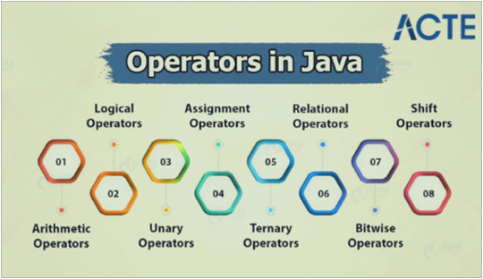
There As Many Types of Operators in Java As Follows:

Arithmetic Operators

Logical Operators

Unary Operators

Assignment Operators

Ternary Operators

Relational Operators

Bitwise Operators

Shift Operators

Arithmetic Operators:

Arithmetic operators in Java facilitate the execution of mathematical expressions, akin to their use in algebra. Java offers operators for five fundamental arithmetic computations: addition, subtraction, multiplication, division, and calculating the remainder. These operations are denoted by the symbols +, -, *, /, and %, respectively. Each of these operators functions as a binary operator, necessitating two values (operands) to carry out the calculations.

Addition (+):

The addition operator (+) in arithmetic performs the task of summing the values of its operands, resulting in the addition of the two values. The operands involved can be of various types, including integer (int, short, byte, long, double) or floating-point (float and double) types.

Subtraction (-):The subtraction operator (-) in Java subtracts the second operand from the first. This operator can work with operands of integer or float types.

Multiplication (*):In Java, the multiplication operator (*) is used to multiply the values of its operands. These operands can be of either integer or float types.

Division (/):In Java, the division operator (/) is used to divide the first operand by the second. The operands may be of either integer or float types.

Modulus (%):The modulus operator (%) in Java computes the remainder of the division of its first operand by the second operand. It essentially finds the modulus of the first operand with respect to the second operand.

Logical Operators in Java

Logical operators, also referred to as conditional operators, are essential for evaluating boolean expressions in complex decision-making scenarios. They generate a boolean value (true or false) as output.

In Java, there are three types of logical or conditional operators: && (Logical-AND), || (Logical-OR), and ! (Logical NOT). Among these, && (Logical-AND) and || (Logical-OR) are binary logical operators that operate on two operands or expressions, while ! (Logical NOT) is a unary logical operator that operates on a single operand or expression. Let's explore into each of them in detail:

The Logical AND Operator (&&):

 It combines two expressions (operands) into one expression, evaluating to true only if both of its expressions (operands) are true.

The Logical OR Operator (||):

 This operator also combines two expressions (operands) into one expression, resulting in a true evaluation if either of its expressions (operands) evaluates to true.

The Logical NOT Operator (!):

It is a unary operator that works on a single operand or expression, negating or reversing the truth value of its operand.

Unary Operators:

Unary operators in Java work on a single operand and can be classified into two types:

Unary plus (+):

This operator signifies the identity operation, leaving the operand value unchanged. For instance, if "number1" is 5, then "+number1" remains 5.

Unary minus (-):

This operator changes the value of the operand to its negative. If "number1" is 5, then "-number1" becomes -5.

Increment/Decrement operators (++/--):

Java includes the increment (++) and decrement (--) operators, which increase or decrease the value of the operand by 1. These operators can be used in two forms: pre-increment and post-increment, as well as pre-decrement and post-decrement.

Assignment Operator (=):

In Java, the assignment operator (=) is employed for assigning a value to a variable.

It adheres to the principle of right-to-left associativity, signifying that the value on the right-hand side of the operator is assigned to the variable on the left-hand side.

Thus, it is crucial to declare the value on the right-hand side before using it or ensure that it remains a constant. This operator serves a fundamental purpose in initializing and updating variables within Java programs.

Ternary Operator

The Java ternary operator is designed to streamline and simulate the if-else statement. It consists of a condition followed by a question mark (?).

The pattern involves two expressions separated by a colon (:).

When the condition evaluates to true, the first expression is executed; otherwise, the second expression is executed.

6.   Relational Operators in Java

·        Relational operators in Java facilitate the comparison of numbers and characters, helping to establish the relationship between operands.

·        These operators assess the relation among the operands and yield results in the boolean data type.

·        They play a crucial role in looping and conditional if-else statements. It is worth noting, however, that relational operators do not function on strings.

Certainly, Here Are the Six Relational Operators in Java Along With Their Corresponding Functionalities:

Equal to (==) Operator: Returns true if the left-hand side is equal to the right-hand side; otherwise, it returns false.

Not Equal to (!=) Operator: Returns true if the left-hand side is not equal to the right-hand side; otherwise, it returns false.

Less Than (<) Operator: Returns true if the left-hand side is less than the right-hand side; otherwise, it returns false.

Less Than or Equal to (<=) Operator: Returns true if the left-hand side is less than or equal to the right-hand side; otherwise, it returns false.

Greater Than (>) Operator: Returns true if the left-hand side is greater than the right-hand side; otherwise, it returns false.

Greater Than or Equal to (>=) Operator: Returns true if the left-hand side is greater than or equal to the right-hand side; otherwise, it returns false.

Bitwise Operators in Java :

Bitwise operators in Java are used to manipulate the individual bits of a number. These operators work with integer types, including byte, short, int, and long. Java provides four bitwise operators:

Bitwise AND Operator (&): Performs a Bitwise AND operation on each corresponding pair of bits of its operands, producing a 1 only if both corresponding bits are 1.

Bitwise OR Operator (|): Returns the Bitwise OR operation for each corresponding pair of bits of its operands, resulting in a 1 if at least one of the bits is 1.

Bitwise XOR Operator (^): Produces a 1 if the two bits of the operands are different; otherwise, the result is 0.

Bitwise Complement Operator (~): Inverts the value of each bit of the operand, turning 1s to 0s and 0s to 1s.

You can use these operators to perform various bitwise operations on numbers. The provided code snippet demonstrates the application of these operators in Java.

8. Shift Operators:

Shift operators in Java are used to perform bit manipulation on operands by shifting the bits of the first operand to the right or left. There are three shift operators available in Java:

Signed Left Shift Operator (<<): This operator shifts the bits of a number or operand to the left and fills the vacated bits on the right with 0. It has a similar effect to multiplying the number with a power of two.

Signed Right Shift Operator (>>): The signed right shift operator shifts the bits of the number to the right. The leftmost vacated bits in this operation depend on the sign of the leftmost bit, or the most significant bit (MSB) of the operand. It has an effect similar to dividing the number by a power of two.

Unsigned Right Shift Operator (>>>): The unsigned right shift operator also shifts the bits of the number to the right. In this operation, the leftmost vacated bits are always set to 0, regardless of the sign of the leftmost bit or the most significant bit (MSB).

It's important to note that in Java, the signed right shift operation fills the vacated bits with a sign bit, while the left shift and the unsigned right shift operation fill the vacated bits with zeroes. These operators allow for various bitwise operations and are useful in scenarios where direct manipulation of bits is required.

In Java, apart from the fundamental arithmetic, logical, bitwise, and shift operators, there are several other operators that serve diverse purposes within the language:

• The Dot . Operator:

The dot operator (.) is utilized to access instance members of an object or class members of a class.

• The () Operator:

 The () operator is used for declaring or calling methods or functions. Arguments for a method can be listed between parentheses, and an empty argument list can be specified using () with nothing between them.

• The instance Of Operator:

The instanceof operator is employed for type checking. It verifies whether its first operand is an instance of its second operand, testing whether an object is an instance of a class, a subclass, or an interface.

Having completed my Java training at ACTE Technologies, I highly recommend their program to individuals seeking to enhance their Java skills. With experienced instructors proficient in Java training, they provides a variety of flexible learning options, catering to both online and in-person preferences. In ACTE Technologies, Java program includes certification opportunities and assistance in securing job placements.

[techblog-365]

R AND PYTHON: GRADIENT DESCENT

Gradient descent is one of the popular optimization algorithms. We use it to minimize the first order derivative of the cost function. You can define a cost function using an equation (example: f(x) = 3x2 + 2x+3) , then do the first order derivative for it ( in this case, f `(x)= 6x+2). Then you can randomly initialize value of x and iterate the value with some learning rate (slope), until we reach convergence (we reach local minimum point). For more details, you can refer simple computational example, with python code, given in Wikipedia . I am taking the same concept of Gradient Descent and applying it for simple linear regression. In the above example, we have the equation to represent the line and we are finding the minimum value. However, in the case of linear regression, we have data points, and we come up with the linear equation, that fits these data points. Here, it works by efficiently searching the parameter space to identify optimal parameters i.e,or . intercept(theta0) and slope(theta1). We initialize the algorithm with some theta values and iterate the algorithm to update theta values simultaneously until we reach convergence. These final theta values (parameters or coefficients), when we put it in equation format, represent best regression line. In machine learning, the regression function y = theta0 + theta1x is referred to as a 'hypothesis' function. The idea, just like in Least squares method, here is to minimize the sum of squared errors, represented as a 'cost function'. We minimize cost function to achieve the best regression line. Let us start with simulating data for simple linear regression.

R:

Importing the dummy data we created. setwd("S:\\ANALYTICS\\R_Programming\\Gradient_Descent") N x beta errors # errors errors y data colnames(data) write.csv(data, file = "Data.csv", row.names = FALSE) Below we are considering the above simulated data for the python coding purpose. #Data simulation for python colnames(data) write.csv(data, file = "Data_Python.csv", row.names = FALSE) Looking at the dimension of data this is because we are working on matrix method. Now we change the dimension of x(predictor) and y(response) accordingly to make matrix multiplication possible. create the x- matrix of explanatory variables. Here we are producing a matrix with 1's in 100 rows to make the matrix dimension is such a way that the multiplication is possible. Data head(Data) ## x y ## 1 55.01790 26.34163 ## 2 63.62490 36.61669 ## 3 56.07122 26.69499 ## 4 61.00054 39.82381 ## 5 63.45294 36.48111 ## 6 62.82037 32.28978 dim(Data) ## [1] 100 2 head(Data) ## x y ## 1 55.01790 26.34163 ## 2 63.62490 36.61669 ## 3 56.07122 26.69499 ## 4 61.00054 39.82381 ## 5 63.45294 36.48111 ## 6 62.82037 32.28978 attach(Data) #n a0 = rep(1,100) a1 = Data[,1] b = Data[,2] x y head(x) ## a0 a1 ## [1,] 1 55.01790 ## [2,] 1 63.62490 ## [3,] 1 56.07122 ## [4,] 1 61.00054 ## [5,] 1 63.45294 ## [6,] 1 62.82037 head(y) ## [,1] ## [1,] 26.34163 ## [2,] 36.61669 ## [3,] 26.69499 ## [4,] 39.82381 ## [5,] 36.48111 ## [6,] 32.28978

Derivative Gradient:

Derivative gradient is the next step after simulating the data in which we obtain the initial parameters. For initializing the parameter of hypothesis function, we considered the first order derivative of the cost function in the below function. where m is the total number of training examples and h(x(i)) is the hypothesis function defined like this: Hypothesis Equation For determining the initial gradient values, we have to consider the first derivative of the cost function which shown below. Cost function J(theta0, theta1) Cost Function Initial_Gradient m hypothesis = x %*% t(theta) loss = hypothesis - y x_transpose = t(x) gradient return(t(gradient)) } Here 'i' represents each observation from the data. For the derivative gradient, we are determining the first derivative of the cost function which gives initial coefficients to update through the gradient runner below. This derivative gradient is called by the gradient runner inside the for loop. From the above function results we will get the matrix of thetas (a0 and a1). Now using the gradient runner, we have to iterate through the theta0 and theta1 until convergence.

Gradient runner:

Gradient runner is the iterative process to update the theta values through the below function until it converges to its local minimum of the cost function. Here in this function additional element we are using is learning rate(alpha) which help to converge to local minimum. For our requirement, we considered alpha as 0.0001. Gradient descent is used to minimize the cost function to get the converged theta value matrix which fits the regression line in data. gradient_descent # Initialize the coefficients as matrix theta #theta #learning rate alpha = 0.0001 for (i in 1:Numiterrations) { theta } return(theta) } print(gradient_descent(x, y, 1000)) ## a0 a1 ## [1,] 0.03548202 0.5777683 To speed up the convergence change learning rate or number of iterations. If you consider learning rate as too small it will take more time to converge and if it is high also it will never converge.

Python:

Import all the required packages and the dummy data to run the algorithm. For python, also we are doing it in matrix method. Same steps to be followed in python as we did using R. from numpy import * import numpy as np import random from sklearn.datasets.samples_generator import make_regression import pylab from scipy import stats import pandas as pd import os path = "S:\\ANALYTICS\\R_Programming\\Gradient_Descent" os.chdir(path) points = genfromtxt("Data_Python.csv", delimiter=",", ) a= points[:,0] b= points[:,1] x= np.reshape(a,(len(a),1)) x = np.c_[ np.ones(len(a)), x] # insert column y = b #For determining the initial gradient values, we have to consider the first derivative of the cost function which shown below. Cost function def Initial_Gradient(x, y, theta): m = x.shape[0] hypothesis = np.dot(x, theta) loss = hypothesis - y x_transpose = x.transpose() gradient = (1/m) * np.dot(x_transpose, loss) return(gradient) #Below gradient descent function is to update the theta0 and theta1 values(coefficients of hypothesis equation) with the initial values untill they converge. We are calling the initial theta value matrix inside the for loop. def gradient_descent(alpha, x, y, numIterations): m = x.shape[0] # number of samples theta = np.zeros(2) x_transpose = x.transpose() for iter in range(0, numIterations): hypothesis = np.dot(x, theta) loss = hypothesis - y J = np.sum(loss ** 2) / (2 * m) # cost theta = theta - alpha * Initial_Gradient(x, y, theta) # update return theta #Now to verify the algorithm in R and Python we are providing learning rate and number of iteration to gradient descent to perform. print(gradient_descent(0.0001,x,y,1000)) ## [ 0.03548202 0.57776832] If you observe from the both algorithms we can see they given the same theta values(coefficients) for hypothesis. While understanding, and applying gradient descent algorithm. Hope you can see the syntactical differences to arrive at same results from R and Python. In this blog, we saw writing functions, handling matrices, loops, and several other things in R and Python. See you next time! About Rang Technologies: Headquartered in New Jersey, Rang Technologies has dedicated over a decade delivering innovative solutions and best talent to help businesses get the most out of the latest technologies in their digital transformation journey. Read More...

[ailtrahq]

Azteco raised $6 million in funding, with Block Inc. CEO Jack Dorsey leading the round. The Santa Monica, California-based company aims to accelerate Bitcoin adoption by introducing Bitcoin gift cards. Azteco’s mission to democratize finance Dorsey’s support for Azteco stems from a deep respect for the company’s mission to make life easier for the unbanked population worldwide.  The former Twitter CEO believes that the technology and resources required to make this positive change are available, and Azteco is taking a crucial step in the right direction. Azteco’s core initiative revolves around introducing Bitcoin gift cards, designed to elevate the flagship crypto’s value to the level of traditional fiat currencies like the US dollar.  The ultimate goal is to democratize finance and establish partnerships with companies across the globe, ensuring that Bitcoin spending becomes a mainstream and widely accepted concept, according to Azteco CEO Akin Fernandez. Relying on a third party as the currency issuer can lead to a single point of failure, he says, adding that centralized control of fiat currencies often results in corruption.  Azteco’s solution is to replace this centralized control with a computer program, allowing Bitcoin to operate as a politically and financially neutral global synthetic currency accessible to people worldwide. Azteco’s reach extends to nearly 600,000 payment locations in about 200 countries. Fernandez emphasizes the significant impact this could have, particularly in the United States, where approximately 4.5% of households were unbanked in 2021.  These households lacked access to e-commerce, making it challenging to buy from online retailers like Amazon, obtain bank loans, or engage in electronic money transfers.  Bitcoin can address these issues by providing around-the-clock global access to a seamless financial system with instant fraud-free transactions. Dorsey’s continued support for Bitcoin This recent funding round led by Dorsey is not the first instance of his commitment to the cryptocurrency space.  In June, he committed $5 million to back Bitcoin developers. Dorsey and his team plan to distribute this sum over five years, providing $1 million yearly to Bitcoin-linked initiatives. This shows Dorsey’s dedication to fostering innovation and development within the Bitcoin ecosystem. Beyond funding Bitcoin development, Dorsey has also been actively involved in promoting Africa’s Web3 talent development. He co-founded the Bitcoin non-profit organization Btrust alongside billionaire music mogul Jay-Z.  Recently, Btrust made a strategic move by acquiring Qala, a company focused on training African Bitcoin and Lightning engineers. This acquisition has led to the rebranding of Qala as the Btrust Builders Program, signifying a synergistic effort to advance Bitcoin development on the African continent. The acquisition of Qala was driven by the recognition that while Btrust possessed the financial resources required, it lacked the infrastructure to nurture and develop the African Bitcoin talent pipeline effectively.  This move represents a significant step in bridging the gap and promoting the growth of Web3 expertise in Africa.