#coderlife codingforlife pyhton | Explore Tumblr posts and blogs

Another Program With Python

Data management will need your own variables that will depend on the variables that you've selected and the decisions you made about them.Data management is a part of the research process, that you can and will return to again, and again, as you learn more, and are able to make better decisions.

In [1]:

import pandas as pd import numpy as np import os import matplotlib.pyplot as plt import seaborn

In [2]:

#this function reads data from csv file def read_data(): data = pd.read_csv('/home/data-sci/Desktop/analysis/course/nesarc_pds.csv',low_memory=False) return data

In [3]:

#this function saves the data in a pickle "binary" file so it's faster to deal with it next time we run the script def pickle_data(data): data.to_pickle('cleaned_data.pickle') #this function reads data from the binary .pickle file def get_pickle(): return pd.read_pickle('cleaned_data.pickle')

In [4]:

def the_data(): """this function will check and read the data from the pickle file if not fond it will read the csv file then pickle it""" if os.path.isfile('cleaned_data.pickle'): data = get_pickle() else: data = read_data() pickle_data(data) return data

In [20]:

data = the_data()

In [21]:

data.shape

Out[21]:

(43093, 3008)

In [22]:

data.head()

Out[22]:

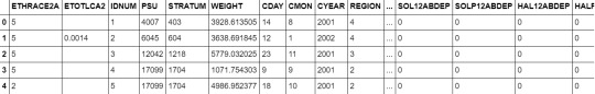
In [102]:

data2 = data[['MARITAL','S1Q4A','AGE','S1Q4B','S1Q6A']] data2 = data2.rename(columns={'MARITAL':'marital','S1Q4A':'age_1st_mar', 'AGE':'age','S1Q4B':'how_mar_ended','S1Q6A':'edu'})

In [103]:

#selecting the wanted range of values #THE RANGE OF WANTED AGES data2['age'] = data2[data2['age'] < 30] #THE RANGE OF WANTED AGES OF FISRT MARRIEGE #convert to numeric so we can subset the values < 25 data2['age_1st_mar'] = pd.to_numeric(data2['age_1st_mar'], errors='ignor')

In [105]:

data2 = data2[data2['age_1st_mar'] < 25 ] data2.age_1st_mar.value_counts()

Out[105]:

21.0 3473 19.0 2999 18.0 2944 20.0 2889 22.0 2652 23.0 2427 24.0 2071 17.0 1249 16.0 758 15.0 304 14.0 150 Name: age_1st_mar, dtype: int64

for simplicity will remap the variable ed to have just 4 levels

below high school education == 0

high school == 1

collage == 2

higher == 3

In [106]:

edu_remap ={1:0,2:0,3:0,4:0,5:0,6:0,7:0,8:1,9:1,10:1,11:1,12:2,13:2,14:3} data2['edu'] = data2['edu'].map(edu_remap)

Print the frequency of the values

In [107]:

def distribution(var_data): """this function will print out the frequency distribution for every variable in the data-frame """ #var_data = pd.to_numeric(var_data, errors='ignore') print("the count of the values in {}".format(var_data.name)) print(var_data.value_counts()) print("the % of every value in the {} variable ".format(var_data.name)) print(var_data.value_counts(normalize=True)) print("-----------------------------------") def print_dist(): # this function loops though the variables and print them out for i in data2.columns: print(distribution(data2[i])) print_dist()

the count of the values in marital 1 13611 4 3793 3 3183 5 977 2 352 Name: marital, dtype: int64 the % of every value in the marital variable 1 0.621053 4 0.173070 3 0.145236 5 0.044579 2 0.016061 Name: marital, dtype: float64 ----------------------------------- None the count of the values in age_1st_mar 21.0 3473 19.0 2999 18.0 2944 20.0 2889 22.0 2652 23.0 2427 24.0 2071 17.0 1249 16.0 758 15.0 304 14.0 150 Name: age_1st_mar, dtype: int64 the % of every value in the age_1st_mar variable 21.0 0.158469 19.0 0.136841 18.0 0.134331 20.0 0.131822 22.0 0.121007 23.0 0.110741 24.0 0.094497 17.0 0.056990 16.0 0.034587 15.0 0.013871 14.0 0.006844 Name: age_1st_mar, dtype: float64 ----------------------------------- None the count of the values in age 1.0 1957 4.0 207 5.0 153 2.0 40 3.0 7 Name: age, dtype: int64 the % of every value in the age variable 1.0 0.827834 4.0 0.087563 5.0 0.064721 2.0 0.016920 3.0 0.002961 Name: age, dtype: float64 ----------------------------------- None the count of the values in how_mar_ended 10459 2 8361 1 2933 3 154 9 9 Name: how_mar_ended, dtype: int64 the % of every value in the how_mar_ended variable 0.477231 2 0.381502 1 0.133829 3 0.007027 9 0.000411 Name: how_mar_ended, dtype: float64 ----------------------------------- None the count of the values in edu 1 13491 0 4527 2 2688 3 1210 Name: edu, dtype: int64 the % of every value in the edu variable 1 0.615578 0 0.206561 2 0.122650 3 0.055211 Name: edu, dtype: float64 ----------------------------------- None

Summary

In [1]:

# ##### marital status # Married 0.48 % | # Living with someone 0.22 % | # Widowed 0.12 % | # Divorced 0.1 % | # Separated 0.03 % | # Never Married 0.03 % | # | # -------------------------------------| # -------------------------------------| # | # ##### AGE AT FIRST MARRIAGE FOR THOSE # WHO MARRY UNDER THE AGE OF 25 | # AGE % | # 21 0.15 % | # 19 0.13 % | # 18 0.13 % | # 20 0.13 % | # 22 0.12 % | # 23 0.11 % | # 24 0.09 % | # 17 0.05 % | # 16 0.03 % | # 15 0.01 % | # 14 0.00 % | # | # -------------------------------------| # -------------------------------------| # | # ##### HOW FIRST MARRIAGE ENDED # Widowed 0.65 % | # Divorced 0.25 % | # Other 0.09 % | # Unknown 0.004% | # Na 0.002% | # | # -------------------------------------| # -------------------------------------| # | # ##### education # high school 0.58 % | # lower than high school 0.18 % | # collage 0.15 % | # ms and higher 0.07 % | # |

1- Re-coding unknown values

from the variable "how_mar_ended" HOW FIRST MARRIAGE ENDED will code the 9 value from Unknown to NaN

In [13]:

data2['how_mar_ended'] = data2['how_mar_ended'].replace(9, np.nan) data2['age_1st_mar'] = data2['age_1st_mar'].replace(99, np.nan)

In [14]:

data2['how_mar_ended'].value_counts(sort=False, dropna=False)

Out[14]:

1 4025 9 98 3 201 2 10803 27966 Name: how_mar_ended, dtype: int64

In [23]:

#pickle the data tp binary .pickle file pickle_data(data2)