#lassoregression python

[gtdk]

Lasso Regression

Lasso regression is a supervised learning method. LASSO actually means Least Absolute Selection and Shrinkage Operator. Lasso imposes a constrain on the model parameters and this causes the regression variables of some coefficients to shrink towards zero. This allows to identify the variables most strongly associated with the target variable by effectively removing unimportant variables from the model.

Let’s try to implement a lasso regression model with python step by step. We will be using diabetes data set of scikit-learn.

1. Split your dataset into train and test sets. You can easily split the diabetes dataset as below.

diabetes_X, diabetes_y = datasets.load_diabetes(return_X_y=True)

X_train = diabetes_X[:-20]

X_test  = diabetes_X[-20:]

y_train = diabetes_y[:-20]

y_test  = diabetes_y[-20:] 

2. Next we can create an object called model that will contain the results of the lasso regression. In parenthesis cv = 10 is added which askes python to use k-fold cross validation with 10 random folds from the training dataset to choose the final statistical model. To fit the lasso regression on the training set we use .fit.

from sklearn.linear_model import LassoLarsCV

model=LassoLarsCV(cv=10, precompute=False).fit(X_train,y_train)

3. Next let’s go ahead and ask python to print the regression coefficients from the model.

model.coef_

output:

array([   0.        , -194.57937837,  514.33452188,  302.88969517,       -101.37105587,    0.        , -234.57718479,    0.        ,        498.24639338,   66.14806771])

As you can see 3 coefficients have shrunk to zeros interpreting that they are unimportant variables. These variables are age,s2 and s4. Also the body mass index and the 5th blood serum has the highest coefficients.

4. Now we can plot the relative importance of the predictor selected at any step of the selection process and how the coefficients changed with addition to new variable and at which step that new variable entered the model.

import numpy as np

# plot coefficient progression

m_log_alphas = -np.log10(model.alphas_)

ax = plt.gca()plt.plot(m_log_alphas, model.coef_path_.T)

plt.axvline(-np.log10(model.alpha_), linestyle='--', color='k', label='alpha CV')

plt.ylabel('Regression Coefficients')

plt.xlabel('-log(alpha)')

plt.title('Regression Coefficients Progression for Lasso Paths')

Here the green line represents the body mass index which has the highest regression coefficient value. The yellow line is the s5.  

5. Another important plot is the one that shows the changes in mean square error when the penalty parameter alpha change at each step.

# plot mean square error for each fold

m_log_alphascv = -np.log10(model.cv_alphas_)

plt.figure()

plt.plot(m_log_alphascv, model.mse_path_, ':')

plt.plot(m_log_alphascv, model.mse_path_.mean(axis=-1), 'k', label='Average across the folds', linewidth=2)

plt.axvline(-np.log10(model.alpha_), linestyle='--', color='k', label='alpha CV')

plt.legend()

plt.xlabel('-log(alpha)')

plt.ylabel('Mean squared error')

plt.title('Mean squared error on each fold')

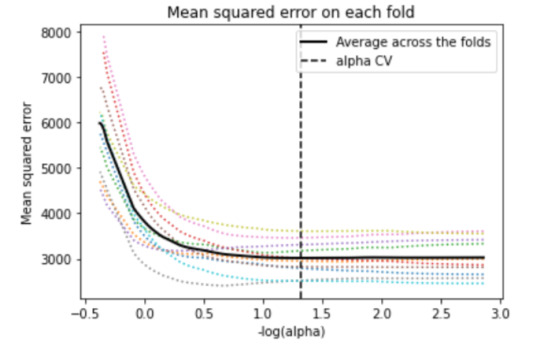
We can see that there is variability across the individual cross-validation folds in the training data set, but the change in the mean square error as variables are added to the model follows the same pattern for each fold. Initially it decreases rapidly and then levels off to a point at which adding more predictors doesn't lead to much reduction in the mean square error. This is to be expected as model complexity increases.

6.  We can also print the average mean square error in the r square for the proportion of variance in school connectedness.   

# MSE from training and test data

from sklearn.metrics import mean_squared_error

train_error = mean_squared_error(y_train, model.predict(X_train))

test_error = mean_squared_error(y_test, model.predict(X_test))

print ('training data MSE - ', train_error)

print ('test data MSE - ', test_error)

# R-square from training and test data

rsquared_train=model.score(X_train,y_train)

rsquared_test=model.score(X_test,y_test)

print ('training data R-square',rsquared_train)

print ('test data R-square',rsquared_test)

7.  At each step of the estimation process, when a new predictor is entered into the model, the mean-square error for the validation fold is calculated for each of the other nine folds and then averaged. The model that produces the lowest mean-square error is selected by Python as the best model to validate using the test dataset.