#newcluster

[jpp--blog]

week4_K-MeansClusterAnalysis

1.- Python Source Code

# -*- coding: utf-8 -*-

from pandas import Series, DataFrame

import pandas as pd

import numpy as np

import os

import matplotlib.pylab as plt

from sklearn.model_selection import train_test_split

from sklearn import preprocessing

from sklearn.cluster import KMeans

from scipy.spatial.distance import cdist

from sklearn.decomposition import PCA

import statsmodels.formula.api as smf

import statsmodels.stats.multicomp as multi

os.chdir("/home/fas-uae/Documents/curso/w4")

# Load the data

data = pd.read_csv("../tree_addhealth.csv")

# Upper-case all DataFrame column names

data.columns = map(str.upper, data.columns)

# Data Management

dataset = data.dropna()

# Subset clustering variables

cluster=dataset[['ALCEVR1','MAREVER1','ALCPROBS1','DEVIANT1','VIOL1','DEP1',

'ESTEEM1','SCHCONN1','PARACTV', 'PARPRES','FAMCONCT']]

cluster.describe()

# Standardize clustering variables to have mean=0 and sd=1

clustervar=cluster.copy()

clustervar['ALCEVR1']=preprocessing.scale(clustervar['ALCEVR1'].astype('float64'))

clustervar['ALCPROBS1']=preprocessing.scale(clustervar['ALCPROBS1'].astype('float64'))

clustervar['MAREVER1']=preprocessing.scale(clustervar['MAREVER1'].astype('float64'))

clustervar['DEP1']=preprocessing.scale(clustervar['DEP1'].astype('float64'))

clustervar['ESTEEM1']=preprocessing.scale(clustervar['ESTEEM1'].astype('float64'))

clustervar['VIOL1']=preprocessing.scale(clustervar['VIOL1'].astype('float64'))

clustervar['DEVIANT1']=preprocessing.scale(clustervar['DEVIANT1'].astype('float64'))

clustervar['FAMCONCT']=preprocessing.scale(clustervar['FAMCONCT'].astype('float64'))

clustervar['SCHCONN1']=preprocessing.scale(clustervar['SCHCONN1'].astype('float64'))

clustervar['PARACTV']=preprocessing.scale(clustervar['PARACTV'].astype('float64'))

clustervar['PARPRES']=preprocessing.scale(clustervar['PARPRES'].astype('float64'))

# Split data into train and test sets

cluster_train, cluster_test = train_test_split(clustervar, test_size=.3, random_state=328)

# k-means cluster analysis for 1-9 clusters                                                          

clusters=range(1,10)

meandist=[]

for k in clusters:

   model=KMeans(n_clusters=k)

   model.fit(cluster_train)

   clusassign=model.predict(cluster_train)

   meandist.append(sum(np.min(cdist(cluster_train, model.cluster_centers_, 'euclidean'), axis=1))

   / cluster_train.shape[0])

'''

Plot average distance from observations from the cluster centroid

to use the Elbow Method to identify number of clusters to choose

'''

plt.plot(clusters, meandist)

plt.xlabel('Number of clusters')

plt.ylabel('Average distance')

plt.title('Selecting K with the Elbow Method')

# Interpret 3 cluster solution

model3=KMeans(n_clusters=3)

model3.fit(cluster_train)

clusassign=model3.predict(cluster_train)

pca_2 = PCA(2)

plot_columns = pca_2.fit_transform(cluster_train)

plt.scatter(x=plot_columns[:,0], y=plot_columns[:,1], c=model3.labels_,)

plt.xlabel('Canonical variable 1')

plt.ylabel('Canonical variable 2')

plt.title('Scatterplot of Canonical Variables for 3 Clusters')

'''

BEGIN multiple steps to merge cluster assignment with clustering variables to examine

cluster variable means by cluster

'''

# Create a unique identifier variable from the index for the

# cluster training data to merge with the cluster assignment variable

cluster_train.reset_index(level=0, inplace=True)

# Create a list that has the new index variable

clusterList=list(cluster_train['index'])

# Create a list of cluster assignments

labels=list(model3.labels_)

# Combine index variable list with cluster assignment list into a dictionary

newList=dict(zip(clusterList, labels))

newList

# Convert newList dictionary to a dataframe

newCluster=DataFrame.from_dict(newList, orient='index')

newCluster

# Rename the cluster assignment column

newCluster.columns = ['cluster']

# Now do the same for the cluster assignment variable

# create a unique identifier variable from the index for the

# cluster assignment dataframe

# to merge with cluster training data

newCluster.reset_index(level=0, inplace=True)

# Merge the cluster assignment dataframe with the cluster training variable dataframe

# by the index variable

merged_train=pd.merge(cluster_train, newCluster, on='index')

merged_train.head(n=100)

# Cluster frequencies

merged_train.cluster.value_counts()

'''

FINALLY multiple steps to merge cluster assignment with clustering variables to examine

cluster variable means by cluster

'''

# FINALLY calculate clustering variable means by cluster

clustergrp = merged_train.groupby('cluster').mean()

print ('Clustering variable means by cluster')

print(clustergrp)

# Validate clusters in training data by examining cluster differences in GPA using ANOVA

# first have to merge GPA with clustering variables and cluster assignment data

gpa_data=dataset['GPA1']

# Split GPA data into train and test sets

gpa_train, gpa_test = train_test_split(gpa_data, test_size=.3, random_state=328)

gpa_train1=pd.DataFrame(gpa_train)

gpa_train1.reset_index(level=0, inplace=True)

merged_train_all=pd.merge(gpa_train1, merged_train, on='index')

sub1 = merged_train_all[['GPA1', 'cluster']].dropna()

gpamod = smf.ols(formula='GPA1 ~ C(cluster)', data=sub1).fit()

print (gpamod.summary())

print ('Means for GPA by cluster')

m1= sub1.groupby('cluster').mean()

print (m1)

print ('Standard deviations for GPA by cluster')

m2= sub1.groupby('cluster').std()

print (m2)

mc1 = multi.MultiComparison(sub1['GPA1'], sub1['cluster'])

res1 = mc1.tukeyhsd()

print(res1.summary())

# Plot clusters

plt.show()

2.- Output

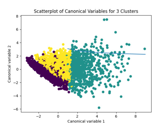
Figure 1: Plot_ScatterplotOfCanonicalVariablesFor3Clusters

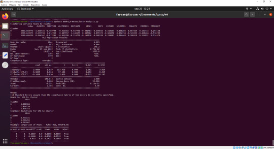
Figure 2: console_K-MeansClusterAnalysis

3.- Interpretation

After the analysis, 3 types of adolescents are considered in the cluster:

Cluster 0 - most likely to have used alcohol

Cluster 1 - most problematic adolescents

Cluster 2 - least problematic adolescents

As part of the analysis, it was observed that adolescents in cluster (the most problematic group) had the lowest GPA of 2.4147; adolescents in cluster 2 (least problematic group), had the highest GPA of 3.001.

In addition, as part of the test, it was observed that the clusters differed significantly in the standard deviation of GPA from their mean GPA value. It can be seen that, for the standard deviation GPA, the difference between cluster 0 and cluster 2 is much smaller than both with cluster 1.

Part of these results can also be seen in the graph above.

[sellygrandbatavia]

*Cluster Pelican* . Terdiri dari 3 type, yaitu Philodendron dengan LB/LT 51/60 , Plumeria dengan LB/LT 46/60 dan Polianthes dengan LB/LT 36/60, Utility Underground, Double Dinding, Security Cluster dan masih banyak lagi kelebihan dan fasilitas dari Cluster Pelican. . Akses Transportasi* -+ 30 Menit Gerbang Tol Cikupa -+ 40 Menit Bandara Soeta -+ 40 Menit Stasiun Tangerang . . Dapatkan Segera Unit Anda Sekarang Juga!!! Info produk: Wa hp 0813.1665.9770 http://bit.ly/tanyainfoprodukpurijayagrandbatavia www.purijayatangerang.com . #clusterpelican #newrelease #bataviaamore #somarchfun #newcluster #premiumcluster #purijaya #bataviaicon #jayarealproperty #grandbatavia #pasarkemis #tangerang #rumah2lantai #rumahmurah #rumahmurahtangerang #rumahpasarkemis #rumahtangerang #rumahtangerangmurah #rumahtangerangdijual #perumahanpasarkemis #perumahanbaru #perumahantangerang #perumahanditangerang #inforumahtangerang #inforumah #jualrumahtangerang #jualrumahtangerangmurah #jualrumahmurah https://www.instagram.com/p/CPUxXmBD4Mc/?utm_medium=tumblr

[sutisnaproperty]

Repost By bsalandofficial: Karena banyaknya permintaan dari konsumen Perumahan #KanaPark @Legok Serpong, akan segera membuka Cluster HANA untuk memenuhi permintaan pasar . Dengan design baru yang modern dan elegan, penghuni Cluster Hana dapat menikmati fasilitas yang lengkap, salah satunya adalah Sports Club Kana Park untuk mendukung gaya hidup sehat anda. . Ayo segera daftar dan dapatkan harga perdana langsung dari BSA LAND, developer dengan track record yang baik dan terpercaya . Informasi lebih lanjut hubungi faris marketing inhouse 087782070518 (whatsapp) atur janjian yuk ma TRISNA DI KANTOR PEMASARAN KANA PARK . Jl. Rancaiyuh Babat Kec. Legok Tangerang Banten #BSALand #BSAproject #KanaPark #Legok #Serpong #newcluster #bebasbanjir #carirumah #rumahkpr #fasilitaslengkap #inforumahtangerang #infotangsel #investasi #properti #cicilanringan (di Kana Park BSA Land) https://www.instagram.com/p/B8v63xsnSfK/?igshid=186tgjmet9ved

[lenytjan-blog]

Rumah bukan sekedar hunian Rumah adalah sebuah pencapaian So... booking segera unit di THE GREEN PADASUKA pembelian Nomor Urut Pemesanan 1 juta tanpa resiko 2 lantai dgn 3 kamar tidur Info segera : LENY TJAN 081 338 161 288 www.supermarketpropertibandung.com #rumahbaru #rumahidaman #rumahideal #rumahkeren #rumahku #rumahcom #rumah123 #rumahkredit #rumahdijual #rumah #perumahan #newcluster #padasuka #greenpadasuka #bukitmoko #infowisata #saungudjo #surapaticore #g4nproperty #ganproperti #instagood #instadaily #cityview #bestpicture #home #housing #realestate #kreditrumah #rumahminimalis #compacthouse #happy #love #like #like4like #followme #me #bandungsatu #bandungjuara #jabar1 #infowisata #infobandung #inforumah

[hartomok]

#newcluster #cluster #burgundy #burgundyresidence #summareconbekasi #summarecon #bekasi #westjava #indonesia Start from 1,079 M-an Link brochure : http://goo.gl/pr1rcv Prosedur pemesanan : 1. FC KTP, NPWP dan KK 2. Commitmet fee 5 juta/unit 3. 1 ktp max 2 unit 4. Launching 20 Mei 2017 5. Handover 24 bulan setelah PPJB Untuk informasi lebih lanjut hubungi : #harto #firstchoicebekasi #firstchoice #bekasi #propertyagent #property #agent #agenproperti Email : harto.mok@gmail.com @rumahcom : http://www.rumah.com/listing-properti/12916031 (di Kota Summarecon Bekasi)

[globalmediacampaign]

Using Volume Snapshot/Clone in Kubernetes

One of the most exciting storage-related features in Kubernetes is Volume snapshot and clone. It allows you to take a snapshot of data volume and later to clone into a new volume, which opens a variety of possibilities like instant backups or testing upgrades. This feature also brings Kubernetes deployments close to cloud providers, which allow you to get volume snapshots with one click. Word of caution: for the database, it still might be required to apply fsfreeze and FLUSH TABLES WITH READ LOCK or LOCK BINLOG FOR BACKUP. It is much easier in MySQL 8 now, because as with atomic DDL, MySQL 8 should provide crash-safe consistent snapshots without additional locking. Let’s review how we can use this feature with Google Cloud Kubernetes Engine and Percona Kubernetes Operator for XtraDB Cluster. First, the snapshot feature is still beta, so it is not available by default. You need to use GKE version 1.14 or later and you need to have the following enabled in your GKE: https://cloud.google.com/kubernetes-engine/docs/how-to/persistent-volumes/gce-pd-csi-driver#enabling_on_a_new_cluster. It is done by enabling “Compute Engine persistent disk CSI Driver“. Now we need to create a Cluster using storageClassName: standard-rwo for PersistentVolumeClaims. So the relevant part in the resource definition looks like this: persistentVolumeClaim: storageClassName: standard-rwo accessModes: [ "ReadWriteOnce" ] resources: requests: storage: 11Gi Let’s assume we have cluster1 running: NAME READY STATUS RESTARTS AGE cluster1-haproxy-0 2/2 Running 0 49m cluster1-haproxy-1 2/2 Running 0 48m cluster1-haproxy-2 2/2 Running 0 48m cluster1-pxc-0 1/1 Running 0 50m cluster1-pxc-1 1/1 Running 0 48m cluster1-pxc-2 1/1 Running 0 47m percona-xtradb-cluster-operator-79d786dcfb-btkw2 1/1 Running 0 5h34m And we want to clone a cluster into a new cluster, provisioning with the same dataset. Of course, it can be done using backup into a new volume, but snapshot and clone allow for achieving this much easier. There are still some additional required steps, I will list them as a Cheat Sheet. 1. Create VolumeSnapshotClass (I am not sure why this one is not present by default) apiVersion: snapshot.storage.k8s.io/v1beta1 kind: VolumeSnapshotClass metadata: name: onesc driver: pd.csi.storage.gke.io deletionPolicy: Delete 2. Create snapshot apiVersion: snapshot.storage.k8s.io/v1beta1 kind: VolumeSnapshot metadata: name: snapshot-for-newcluster spec: volumeSnapshotClassName: onesc source: persistentVolumeClaimName: datadir-cluster1-pxc-0 3. Clone into a new volume Here I should note that we need to use the following as volume name convention used by Percona XtraDB Cluster Operator, it is: datadir--pxc-0 Where CLUSTERNAME is the name used when we create clusters. So now we can clone snapshot into a volume: datadir-newcluster-pxc-0 Where newcluster is the name of the new cluster. apiVersion: v1 kind: PersistentVolumeClaim metadata: name: datadir-newcluster-pxc-0 spec: dataSource: name: snapshot-for-newcluster kind: VolumeSnapshot apiGroup: snapshot.storage.k8s.io storageClassName: standard-rwo accessModes: - ReadWriteOnce resources: requests: storage: 11Gi Important: the volume spec in storageClassName and accessModes and storage size should match the original volume. After volume claim created, now we can start newcluster, however, there is still a caveat; we need to use: forceUnsafeBootstrap: true Because otherwise, Percona XtraDB Cluster will think the data from the snapshot was not after clean shutdown (which is true) and will refuse to start. There is still some limitation to this approach, which you may find inconvenient: the volume can be cloned in only the same namespace, so it can’t be easily transferred from the PRODUCTION namespace into the QA namespace. Though it still can be done but will require some extra steps and admin Kubernetes privileges, I will show how in the following blog posts. https://www.percona.com/blog/2020/10/22/using-volume-snapshot-clone-in-kubernetes/

[sellygrandbatavia]

*Cluster Pelican* . Terdiri dari 3 type, yaitu Philodendron dengan LB/LT 51/60 , Plumeria dengan LB/LT 46/60 dan Polianthes dengan LB/LT 36/60, Utility Underground, Double Dinding, Security Cluster dan masih banyak lagi kelebihan dan fasilitas dari Cluster Pelican. . Akses Transportasi* -+ 30 Menit Gerbang Tol Cikupa -+ 40 Menit Bandara Soeta -+ 40 Menit Stasiun Tangerang . . Dapatkan Segera Unit Anda Sekarang Juga!!! Info produk: Wa hp 0813.1665.9770 http://bit.ly/tanyainfoprodukpurijayagrandbatavia www.purijayatangerang.com . #clusterpelican #newrelease #bataviaamore #somarchfun #newcluster #premiumcluster #purijaya #bataviaicon #jayarealproperty #grandbatavia #pasarkemis #tangerang #rumah2lantai #rumahmurah #rumahmurahtangerang #rumahpasarkemis #rumahtangerang #rumahtangerangmurah #rumahtangerangdijual #perumahanpasarkemis #perumahanbaru #perumahantangerang #perumahanditangerang #inforumahtangerang #inforumah #jualrumahtangerang #jualrumahtangerangmurah #jualrumahmurah (di McD Grand Batavia) https://www.instagram.com/p/CPUxSXdFahL/?utm_medium=tumblr

[sellygrandbatavia]

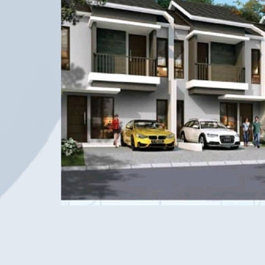
Yuk dapatkan infonya langsung sebelum kehabisan lagi. . Murah guys rumah komersil konsep 2 lantai . Harga yang ditawarkan start dari 500 JTn dan DP bisa dicicil hingga 18-24 bulan. Grab it fast survey sekarang juga . . Dapatkan Segera Unit Anda Sekarang Juga!!! Info produk: Inget Selly ya kk WA/hp 0813.1665.9770 www.purijayatangerang.com . #newrelease #bataviaamore #newcluster #premiumcluster #purijaya #bataviaicon #clusterpelican #jayarealproperty #grandbatavia #tangerang #tangerang #rumah2lantai #rumahmurahready #rumahmurahtangerang #bumiindah #rumahtangerang #kotasuter #rumahtangerangdijual #tamanwalet #gajahtunggal #perumahantangerang #perumahanditangerang #inforumahtangerang #inforumah #rumahkomersil #jualrumahgrandbatavia #jualrumahmurah #clusteramore #sellypurijaya #marketingpurijaya #stockready (di Tangerang) https://www.instagram.com/p/CPUmo2iDIKe/?utm_medium=tumblr

[sellygrandbatavia]

Yuk dapatkan infonya langsung sebelum kehabisan lagi. . Murah guys rumah komersil konsep 2 lantai . Tipe Azalea menawarkan tanah 60 bangunan 46 lebar 5x12m, tipe ini memiliki 2 KT dan 2 KM . . Dapatkan Segera Unit Anda Sekarang Juga!!! Info produk: Inget Selly ya kk WA/hp 0813.1665.9770 www.purijayatangerang.com . #newrelease #bataviaamore #newcluster #premiumcluster #purijaya #bataviaicon #clusterpelican #jayarealproperty #grandbatavia #tangerang #tangerang #rumah2lantai #rumahmurahready #rumahmurahtangerang #bumiindah #rumahtangerang #kotasuter #rumahtangerangdijual #tamanwalet #gajahtunggal #perumahantangerang #perumahanditangerang #inforumahtangerang #inforumah #rumahkomersil #jualrumahgrandbatavia #jualrumahmurah #clusteramore #sellypurijaya #marketingpurijaya #stockready (di Taman Walet, Pasar Kemis) https://www.instagram.com/p/CPUmdoSjv54/?utm_medium=tumblr

[sellygrandbatavia]

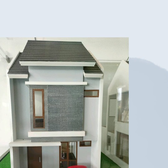
Yuk dapatkan infonya langsung sebelum kehabisan lagi. . Murah guys rumah komersil konsep 2 lantai . Tipe Azalea menawarkan tanah 60 bangunan 46 lebar 5x12m, tipe ini memiliki 2 KT dan 2 KM . . Dapatkan Segera Unit Anda Sekarang Juga!!! Info produk: Inget Selly ya kk WA/hp 0813.1665.9770 www.purijayatangerang.com . #newrelease #bataviaamore #newcluster #premiumcluster #purijaya #bataviaicon #home #jayarealproperty #grandbatavia #designrumah #rumah2lantai #rumahmurahready #rumahmurahtangerang #bumiindah #rumahtangerang #kotasuter #rumahtangerangdijual #homedecor #rumahminimalis #rumahminimalismodern #perumahanditangerang #inforumahtangerang #inforumah #rumahkomersil #jualrumahgrandbatavia #jualrumahmurah #clusteramore #sellypurijaya #marketingpurijaya #stockready (di Grand batavia) https://www.instagram.com/p/CPUmacIDDij/?utm_medium=tumblr

[sellygrandbatavia]

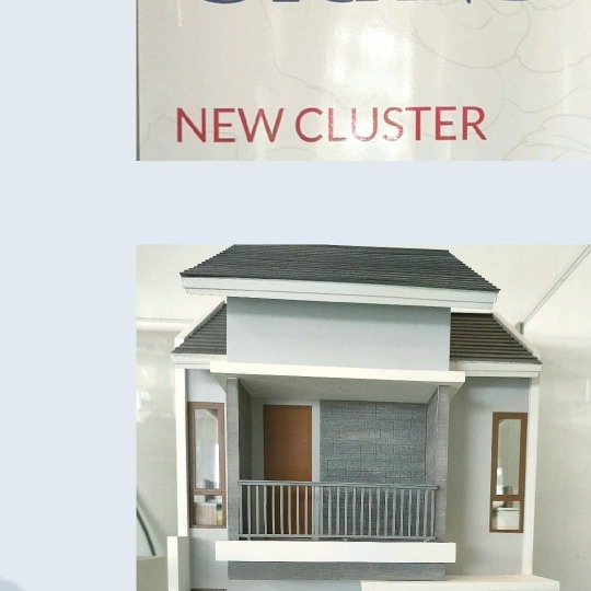
Yuk dapatkan infonya langsung sebelum kehabisan lagi. . Murah guys rumah komersil konsep 2 lantai ada konsep balkon . Tipe tanah ada 72 bangunan 63 lebar 6x12m, tipe ini memiliki 3 KT dan 2 KM . . Dapatkan Segera Unit Anda Sekarang Juga!!! Info produk: Inget Selly ya kk WA/hp 0813.1665.9770 www.purijayatangerang.com . #newrelease #bataviaamore #newcluster #premiumcluster #purijaya #bataviaicon #clusterpelican #jayarealproperty #grandbatavia #tangerang #tangerang #rumah2lantai #rumahmurahready #rumahmurahtangerang #bumiindah #rumahtangerang #kotasutera #rumahtangerangdijual #tamanwalet #property #lavonswancity #lavon #perumahanditangerang #inforumahtangerang #rumahkomersil #jualrumahgrandbatavia #jualrumahmurah #clusteramore #sellypurijaya #marketingpurijaya #stockready (di Grand batavia) https://www.instagram.com/p/CPUmFh5jjEL/?utm_medium=tumblr

[sellygrandbatavia]

Yuk dapatkan infonya langsung sebelum kehabisan lagi. . Murah guys rumah komersil konsep 2 lantai . Tipe tanah ada 72 bangunan 63 lebar 6x12m, tipe ini memiliki 3 KT dan 2 KM . . Dapatkan Segera Unit Anda Sekarang Juga!!! Info produk: Inget Selly ya kk WA/hp 0813.1665.9770 www.purijayatangerang.com . #newrelease #bataviaamore #newcluster #premiumcluster #purijaya #bataviaicon #clusterpelican #jayarealproperty #grandbatavia #taehyung #rumah2lantai #rumahmurahready #rumahmurahtangerang #bumiindah #rumahtangerang #kotasutera #rumahtangerangdijual #tamanwalet #panarub #perumahantangerang #perumahanditangerang #inforumahtangerang #inforumah #rumahkomersil #jualrumahgrandbatavia #jualrumahmurah #clusteramore #sellypurijaya #marketingpurijaya #stockready (di Grand batavia) https://www.instagram.com/p/CPUl5fejD_2/?utm_medium=tumblr

[sellygrandbatavia]

Yuk dapatkan infonya langsung sebelum kehabisan lagi. . Murah guys rumah komersil konsep 2 lantai . Harga start dari 500 jtan DP bisa dicicil hingga 18-24 bulan, tersedia 2 type guys -Tipe Alamanda 63/72 -Tipe Azalea 46/60 . . Dapatkan Segera Unit Anda Sekarang Juga!!! Info produk: Inget Selly ya kk WA 0813 16659770 www.purijayatangerang.com . #newrelease #bataviaamore #newcluster #premiumcluster #purijaya #bataviaicon #clusterpelican #jayarealproperty #grandbatavia #pasarkemis #tangerang #rumah2lantai #rumahmurah #rumahmurahtangerang #rumahpasarkemis #rumahtangerang #rumahtangerangmurah #rumahtangerangdijual #perumahanpasarkemis #perumahanbaru #perumahantangerang #perumahanditangerang #inforumahtangerang #inforumah #jualrumahtangerang #jualrumahtangerangmurah #jualrumahmurah #clusteramore #sellypurijaya #marketingpurijaya (di Grand batavia) https://www.instagram.com/p/CPUk_k0D9uf/?utm_medium=tumblr

[sellygrandbatavia]

Realease cluster Amore menggunakan spesifikasi batu bata merah, double dinding, listrik bawah tanah, dan listrik 2.200 Watt . -Tipe Alamanda 63/72 -Tipe Azalea 46/60 . . Dapatkan Segera Unit Anda Sekarang Juga!!! Info produk: Inget Selly ya kk WA 0813 16659770 www.purijayatangerang.com . #newrelease #bataviaamore #newcluster #premiumcluster #purijaya #bataviaicon #clusterpelican #jayarealproperty #grandbatavia #pasarkemis #tangerang #rumah2lantai #rumahmurah #rumahmurahtangerang #rumahpasarkemis #rumahtangerang #rumahtangerangmurah #rumahtangerangdijual #perumahanpasarkemis #perumahanbaru #perumahantangerang #perumahanditangerang #inforumahtangerang #inforumah #jualrumahtangerang #jualrumahtangerangmurah #jualrumahmurah #clusteramore #sellypurijaya (di Grand batavia) https://www.instagram.com/p/CPUkwVDDRVB/?utm_medium=tumblr

[sellygrandbatavia]

Masih belum nemu rumah yang pas dengan selera kamu? Pilih Grand Batavia Aja! . Grand Batavia berlokasi di Jl. Raya Cadas-Kukun, Ps. Kemis. Memiliki lokasi yang cukup strategis dengan akses dari dan menuju beberapa tempat transportasi yang cukup mudah. - Dari dan menuju Gerbang Tol Cikupa -+ 30 Menit - Dari dan menuju Bandara Soeta -+ 40 Menit - Dari dan menuju Stasiun Tangerang -+ 40 Menit. . . Info produk: Wa.me/6281316657990 www.purijayatangerang.com . #newrelease #bataviaamore #somarchfun #newcluster #premiumcluster #purijaya #bataviaicon #clusterpelican #jayarealproperty #grandbatavia #pasarkemis #tangerang #rumah2lantai #rumahmurah #rumahmurahtangerang #rumahpasarkemis #rumahtangerang #rumahtangerangmurah #rumahtangerangdijual #perumahanpasarkemis #perumahanbaru #perumahantangerang #perumahanditangerang #inforumahtangerang #inforumah #jualrumahtangerang #jualrumahtangerangmurah #jualrumahmurahtangerang (di Puri Jaya Grand Batavia) https://www.instagram.com/p/CPM4wiBDvTo/?utm_medium=tumblr

[sellygrandbatavia]

In Update progres pembangunan Batavia Icon Mei 2021. Pembangunan beberapa unit sudah terlihat memasuki progres 40% up. . . Dapatkan Segera Unit Anda Sekarang Juga!!! Info produk: WA 0856.1017.220 www.purijayatangerang.com . #newrelease #bataviaamore #newcluster #premiumcluster #purijaya #bataviaicon #clusterpelican #jayarealproperty #grandbatavia #pasarkemis #tangerang #rumah2lantai #rumahmurah #rumahmurahtangerang #rumahpasarkemis #rumahtangerang #rumahtangerangmurah #rumahtangerangdijual #perumahanpasarkemis #perumahanbaru #perumahantangerang #perumahanditangerang #inforumahtangerang #inforumah #jualrumahtangerang #jualrumahtangerangmurah #jualrumahmurah https://www.instagram.com/p/CPKGU9HjwpR/?utm_medium=tumblr