#that is exactly the case that the minimum polynomial is linear

[bubbloquacious]

Jacobson's Basic algebra 1 gives such a nice argument for why algebraic numbers have minimum polymials, making it a corollary of the fact that polynomial rings over fields are principal ideal domains. Consider a field extension E/F (i.e. a field E that contains a field F). For any u ∈ E we have in E the subring F[u] and the subfield F(u). These are defined as the smallest subring and subfield of E respectively that contain both F and u. If E = F(u) for some u ∈ E, then E/F is called a simple field extension.

Let F(u)/F be an arbitrary simple field extension. Consider the polynomial ring F[X]. By the universal property of polynomial rings (which is essentially what one means when they say that X is an indeterminate), there is a unique ring homomorphism F[X] -> F(u) that sends any a ∈ F to itself and that sends X to u (you can think of this homomorphism as evaluation of a polynomial at u). If the kernel of this homomorphism is the zero ideal, then F[u] is isomorphic to F[X], so u is transcendental over F. If the kernel is non-zero, then by definition there are non-zero polynomials p ∈ F[X] such that p(u) = 0 in F(u), so u is algebraic over F. Because F[X] is a principal ideal domain, there is a polynomial p that generates the kernel. In other words, p divides all polynomials q such that q(u) = 0 in F(u). Two polynomials (over a field) generate the same ideal if and only if they differ by a constant factor, so there is a unique monic minimum polynomial in F[X] for u.

[catvbroadcast-blog]

Basic RF Definitions and IMD Effects on TV Picture (Distortions and Dynamic Range)

Source: Freeimages.com (Holger Dieterich)

Any active system can be clarified by the power series. This term is right in The very initial approximation, once the machine does not have any memory. Memory effects of an Active system are brought on by a time-varying period reply, which is, subsequently, Manifested at the frequency response. The Phenomenon describes how the phase response is influenced by input power. Under These conditions of memory, the system is clarified by way of a Volterra series. The energy show demonstration here believes AM- to-PM effects just and also the Associated calculation is scalar only, which means an easy polynomial with real coefficients.

System operation for linearity and dynamic range (DR) is measured by the Two tone test forecasting the second-order intercept point (IP2) and third-order intercept point (IP3). Order intersects the linear gain line, as shown in Fig. 9.1. Thus, IP2 Is the virtual point at which in fact the second stimulation line intersects the first-order Linear gain line. In exactly the same style, IP3 and also IPn are all defined. Spectrumwise, this Means that at the ip address, the power level of the spurious intermodulations (IMDs) Are equal to this fundamental signal ability. In community access television (CATV), third-order IMDs are debatable, Since they have reached exactly the exact same frequency of this company. In an narrow-band system, In Terms of a second-order IMD, at an narrow-band system, they’re filtered out; but in CATV system, they Are within the band, using an offset of +1.25 MHz from the channel carrier.

One at 21.25 MHz is CSO_L. Observing the NTSC frequency plan given in Sec. 3.4, it is known that CSO distortions are equally as within the CATV band. Distortions could be filtered outside; in actuality, actually each second-order intermodulation Product could be filtered out in a few instances. Generally, intermodulations along with Spurious-free dynamic range (SFDR) are tested by 2 variations, whilst IP2 and IP3 Are appraised by 2 variations also.

The distortion created by the third-order word in Eq. (9.1) is intriguing since it Relates to the composite triple beat (CTB) in a multi-tone loading and creates the both tones are all equal in amplitude; when substituting this value from Eq. (9.1) And resolving the third-order term working with a few trigonometric identities, a fundamental Tone is produced by the third-order term having an amplitude of both 2.25a3A3. The Third harmonic generated for each frequency is using an amplitude of 0.25a3A3, As in case of one tone.

Cross Modulation Effects

When shooting the IP3 Twotone evaluation, sometimes it can be discovered that the IMD distortion Levels aren’t equal in amplitude as shown at Fig. 9.4. The reason behind this phenomenon is the AM-to-PM conversion consequent From memory effects and fifth-order provisions beats. As a consequence, the IMD Solutions Are not added in period versus frequency. Hence, the characterization of the Device has to be both, by measuring its own AM-to-AM curve also from AM-to-PM, Curve showing the amount of change in the transfer stage of the device for a function Of electricity.

The above relation affects the prestige of second-order IMDs as well. Thus, when Dealing with the two tone evaluation, it may seem to get any station, you can find differences Between its discrete second-order high (DSO), which can be above the highfrequency Test signal company and its particular DSO low, which is beneath the low-frequency Test signal carrier at a specified frequency test, when the input power is varied. This Analysis kind related to memory effects is known as Volterra series analysis.

Multitone CTB Relations

When more than two carriers are Within a station, third-order interference can Be created by the multiplication of three carriers that are fundamental. Back in CATV systems, it Is generally utilized to gauge the distortions with over two signs. Thus, IP3 Stinks to CTB, also IP2 corresponds to CSO. All these CTB spurious signals Are normally 6 dB higher compared to standard two tone evaluation products understood to be Discrete two tone, third-order be at (DTB). The level of CTB is further enhanced By the fact that multiple CTB signs can occur in precisely the exact same frequency group. The number of all CTB signals being clubbed on any Specific channel is Related to the amount of carriers present. Statistics reveals that more CTB interference does occur in the central band.

RF chain lineup is also a significant point when designing any Type of RF or analog Optical receiver. The correct lineup will provide the desirable sound figure 10 log(F) (NF) for your system and thus fulfills CNR functionality, profit, and low distortion, That produce low IMD levels that specify the machine doctor to be quite high. When Designing an RF lineup, there is just a need to be aware of the input power range into the RF string, the required output power from the recipient at its minimum input Power, and also the CNR at the point. The CNR requirement defines the RF chain Max NF. When It Comes to an optical receiver, as will be discussed later on, there Is a necessity to find out the OMI and the optical power scope, the responsivity of The photo detector (PD), in addition to the input impedance at the PD output port In order to derive the input power. Ordinarily, when designing any kind of receiver, the very first phase at the RF Front end (RFFE) ought to really be a low-noise amplifier (LNA), together with high-output P and IP3. These demands stipulate each other, and a compromise The initial phase at the RF chain defines That the RF series NF P1dB and IP3, which results in the recipient’s DR. A typical Lineup of a CATV receiver with an automatic gain control (AGC) attenuator, Voltage variable attenuator (VVA), or digital controlled attenuator (DCA) is Given in Fig.

For more infotmation, please visit https://catvbroadcast.com/news/basic-rf-definitions-and-imd-effects-on-tv-picture-distortions-and-dynamic-range/

[refinery29engineering]

SEO A/B Testing With S.E.O.L. (soul)

[Editor’s Note: This post was originally published on Medium here.]

A/B testing is a standard procedure for using data to inform decision-making in the tech world. Modifications introduced to a product can be compared to either another variation or some baseline, allowing us to understand exactly just how much this modification increases the value of the product or introduces risk. When we see significant positive results, we roll out the change with confidence.

This approach is pretty simple with conversion-based A/B testing: you compare the number of conversions occurring on two variations of a page. Conversions could be any measurable behavior — checkouts, link clicks, impressions on some asset, or reaching a specified destination. The math for this also works out pretty simply: a rate or mean calculation and a p-value calculation on that value.

But the methodology for A/B testing conversion rates doesn’t translate to an SEO context!

First, SEO-based modifications don’t usually affect user behavior; they affect how search bots rank the page. Second, it doesn’t make sense to create 2 different versions of the same page because search rankings are negatively impacted by duplicates. Third, you can’t directly compare test and control groups in an SEO context, because SEO behavior is different for every single page. Lastly, there isn’t a clear conversion metric. With SEO-based testing, in the absence of knowledge of the inner workings of Google’s ranking algorithm, we want to see if our changes affect the volume of traffic we receive from search services like Google. Thus in order to understand how SEO based changes affect traffic, we need to compare the performance after the change to the performance we’d expect. To do so we created SEOL (pronounced soul), the Search Engine Optimization Legitimator.

SEOL Oracle — Prediction vs. Reality

The way SEOL works, is by first fitting a forecasting model to historical data for a group of pages in question. Once the model is fit, the performance of the group of pages is forecasted for the dates from the starting of the intervention (launch date), till the end of the test. Finally, when we have our forecast and we have the data about how it actually performed, we perform tests to measure whether deviations from our expectation (forecast) are statistically significant. If we see significant results in the test group, either positive or negative, and we don’t see the same fluctuations in the control group, we can confidently say that our changes have made an effect. If both groups are affected in the same direction, even if the deviation is significant, we can conclude that the deviation was something systemic, and was not caused by the update in question.

This is typically a 3 part process: group selection, performance forecasting, significance testing. I’d like to explain each one of these steps in more detail.

Group Selection

Before we can perform this analysis we must first select stories to be in the test and control groups. We want to select groups that are the most statistically similar — you can think of this as selecting groups with the highest pearson correlation coefficient. In addition to being correlated, you’d also want them to be in the most similar scale possible, so this you can consider as the minimum Euclidean distance between the two time series (using time step as a dimension). In simpler language, select groups that look/perform the same, as much as possible. We must also be wary of selecting groups that have a similar number of stories in them, each of which perform proportionately similar as well. If the test group has 10 stories, and 5 of them contribute 80% of the performance (ideally each story contributes an equal amount), then there should also be 10 item in the control group, 5 of which contribute 80% of the performance. In addition, avoiding seasonally driven stories is also important. These could perform as outliers, throwing off the results of the test. The purpose of this is to select groups you can be confident will perform similarly, and won’t have any unexpected perturbations to group performance.

SEO Performance Forecasting

The task of forecasting a group of pages performance breaks down into two parts:

Separating the performance data we already have into its behavioral cadence and metric trends

Modeling/forecasting in each component, and recombining them

Let’s start with discussing the decomposition of the performance data.

Below is an illustration of the signal decomposition results. We decompose the signal so that we can model the underlying shape that characterizes the general behavior in the data. This is called making the data stationary (you can learn more about that here). There are various approaches to this, but we stationarized the data by taking a rolling mean of the data, in which any given point represents average of some previous time periods (e.g., a week), and then subtracting that moving average from the vanilla signal. Thus, perturbations due to the ebb and flow of story popularity are cancelled out, leaving behind the natural cadence of weekday/weekend behavior. The moving average is also plotted, on the right, because this is the trend component. The trend represents the popularity of the group’s stories over time.

Now that we’ve decomposed our signal, we have to forecast performance from the intervention date until the end of the dates in the data set. This is done using regression methods. We used Polynomial Regression to model the stationary signal, and linear regression to model the trend.

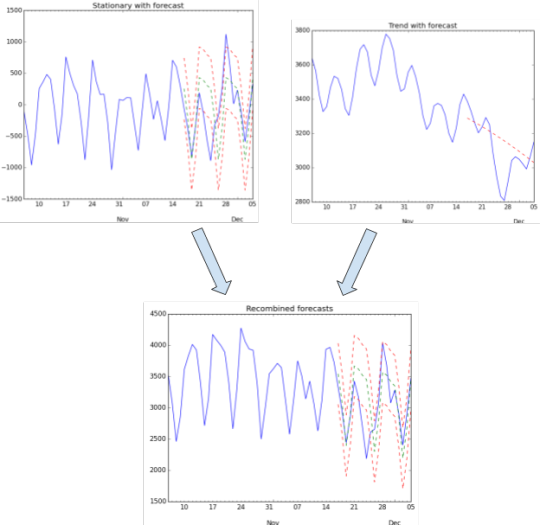
Now that we’ve made forecasts on our decomposed items, we simply sum them to recover our original data. Now that we have our performance data and forecasts, we can perform our statistical tests. Note that we also model what our predictions look like plus and minus 1 standard deviation. This helps us get a sense of the kinds of variations in the reality that should fall into an acceptable range.

Forecast vs. Reality Statistical Significance Testing

Now that we have our data representing the reality of how the pages performed, and our forecast for what we expected in that same time frame, we can perform statistical significance tests to see if our expectation meets the reality or not. For this task we use 2-sided paired t-tests. The paired is designed for before/after testing. Here we use the forecast as our ‘before’ data, and the reality as our ‘after’ data. Here’s a bit more detail:

“Examples for the use are scores of the same set of student in different exams, or repeated sampling from the same units. The test measures whether the average score differs significantly across samples (e.g. exams). If we observe a large p-value, for example greater than 0.05 or 0.1 then we cannot reject the null hypothesis of identical average scores. If the p-value is smaller than the threshold, e.g. 1%, 5% or 10%, then we reject the null hypothesis of equal averages.”

[Quote found here. I’m using this exact software to perform the test]

In addition we also test to see if the reality equals forecast plus/minus 1 standard deviation, and plus/minus ½ standard deviation to get more precision on how the performance actually turned out. So when we perform our paired t-test, for example comparing reality & expectation + 1 standard deviation, we receive a p-value. If the p-value is below 0.05 then we reject the hypothesis that they are equal, otherwise we accept. If the test group has a significant result that the control group does not also have, then we can conclude that there was indeed a real change in the test group.

Post Analysis notes

After the duration of the test period, one may want to inspect how the stories in each group actually performed. If a story had an outlier performance, perhaps due to unforeseeable circumstances, then you may want to remove it from the analysis. For example, David Bowie content got a boost in the time surrounding his death. There’s no way for us to have predicted that, and hence it would alter how our groups perform against the expectation. If this is the case, find the story or stories needing removal, and run the test again. In addition, in the case of online publication, like our business, we found that it makes more sense to analyze only pages (stories) that were published before the test period. Older stories tend to have a trend they follow, making modeling more straight forward and effective. Lastly, try not to perform these types of tests during periods with seasonal effects. For example Christmas and New Years results in dips to our traffic, as I’d expect for most websites, and this causes added difficulty to the modeling process.

Results Overview

We’ve recently completed a big project as a department. Our goal was to move our slideshow template to a new technology stack. This stack included a front and back end, making our pages faster, and adding in some new capabilities, but didn’t change anything else. Meaning we didn’t introduce any changes with the intention of affecting SEO. But before we planned a full release, we wanted to conduct a test on a small set of stories to see if our new template introduced any risk to our product.

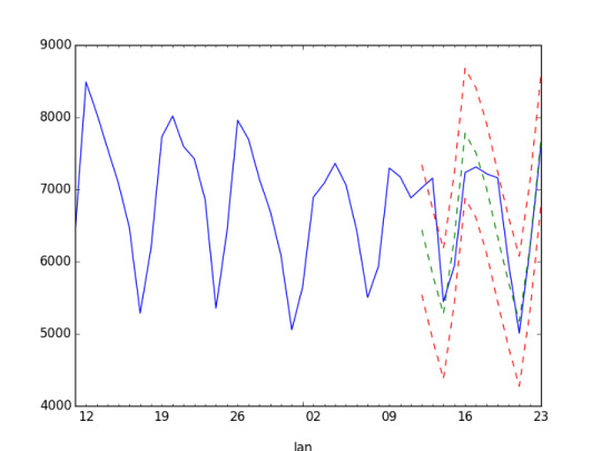
So we chose test and control groups that included about 8000 stories, each of which have little impact on our bottom line (making them somewhat safe to test with), let them run for a couple weeks, and conducted our SEOL analysis. You can see those results below.

Test Group

Actual performance with expectation and +/- 1 standard deviation

standard deviation = 882.672983891

performance = expected + std: pval = 1.05651517695e-05

performance = expected + std/2: pval = 9.58082513196e-09

performance = expected: pval = 0.310003313956

performance = expected — std/2: pval = 3.78494096065e-10

performance = expected — std: pval = 0.000193616202526

Control Group

Actual performance with expectation and +/- 1 standard deviation

performance = expected + std: pval = 0.000571541676843

performance = expected + std/2: pval = 1.28055991188e-09

performance = expected: pval = 0.303194513375

performance = expected — std/2: pval = 7.21701889467e-11

performance = expected — std: pval = 2.45454965489e-05

Interpretation

Both the test and control groups showed that we must accept the hypothesis that performance is at expectation. This means that the new template appeared to perform on par with the old template at garnering organic traffic. This was good news for us, implying that our work didn’t have negative affects on crucial search traffic. This was our goal!

Conclusion

In order to test SEO-related changes we need to evaluate how they perform versus some expectation. Because SEO relates to the behavior of people and products outside of our ecosystem, we can make guesses on how they will perform, and then test against that, but directly comparing them is not a valid test method. This gives us the capability to test any SEO based changes with great detail, and a reliable way to ensure we’re not launching products that hurt us.

So to anyone needing a better way to understand how SEO based changes affect your products, try using an approach like SEOL.

-- Aaron Bernkopf, Data Scientist @ Refinery29