thepandas

[thepandas]

Capstone Project - Draft Results

Univariate Analysis

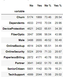
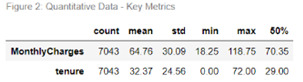
Figure 1 contains frequency counts and distribution percentages for each Yes/No categorical variable including Churn (the response variable). Noticeably the churn variable is skewed where 26.5% of customer have churned and 73.5% have not. Payment Method contains four responses, Electronic check being the highest method at 33.6% and Credit Card the lowest at 21.6% (22.9% Mailed check & 21.9% Bank Transfer). Contract type comprises of three responses, Monthly being the most popular type at 55.0%, followed by Two Year contract at 24.1% and the remaining 20.9% on a One Year contract. For the two quantitative variables, Monthly Charges and Tenure, metrics have been produced in figure 2 – based on these metrics, Monthly Charges exhibits a negative (or left) skew while Tenure demonstrates a positive (or right) skew.

Bivariate analysis

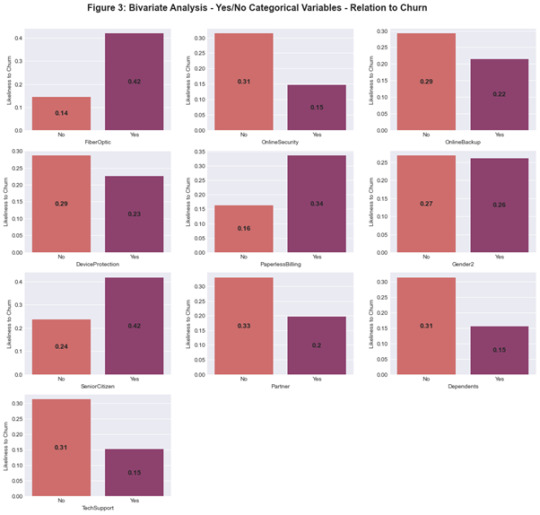
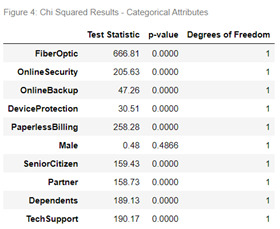
The bivariate analysis for Yes/No Categorical data in relation to the ‘Churn’ response variable is displayed in Figure 3. When a customer has fiber-optic internet they display the highest likeliness to churn based on the Telco Dataset. Figure 4 exhibits the results of the chi squared test of independence for each Yes/No categorical variable in relation to the ‘Churn’ response variable. All predictor variables demonstrated a significant difference in relation to churn except for Male which returned a p-value of 0.4866.

For the contract type variable, each group was tested against another using the Chi squared test of independence where a Bonferroni adjustment was applied to the p-value to be 0.017. All group comparisons showed a significant difference (Likeliness to churn: Month-to-month 43%, One Year 11% and Two Year 3%).

The chi-squared test was applied to the Payment Method variable which has 4 responses and was tested in association to the Churn response variable. The p-value results for each test are exhibited in figure 5. Electronic check has the highest likeliness to churn at 45% then Mailed Check 19%, Bank Transfer 17% and finally credit card 15%.

Analysis of Variance (ANOVA) models were produced for quantitative variables to assess the variance between churned customers and live customers. The model for Monthly Charges showed a significant difference between groups with an F-statistic of 273.5 (1, 7041) and a p value < 0.001. Figure 6 displays a box plot where the median is 79.65 for those that have churned with a lower quartile as 56.15 and an upper quartile of 94.20 (IQR = 38.05). Whereas live customers have a median monthly charge of 64.43 with a lower quartile of 25.10 and upper 88.40 (IQR = 63.3). The figure also includes a bar graph where the average Monthly Charges for a churned customers is 74.44 with a standard deviation of 24.67 as opposed to a live customers with an average charge of 61.27 and a standard deviation of 31.09.

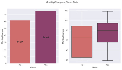
Figure 6: MonthlyCharges – Churn Data

An ANOVA model was produced for Tenure which also showed a significant difference between churned and live customers – F-statistic of 997.3 (1, 7041) and a p value < 0.001. Figure 7 shows churned customers to have an average tenure of 17.98 months with a standard deviation of 19.53. They also have a median of 10.00 months with an upper quartile of 29 months and lower of 2 (IQR = 27). Live Customers have an average tenure of 37.57 months, with a standard deviation of 24.11. The median is 38 months with a lower quartile of 15 months and upper of 61 months (IQR = 46).

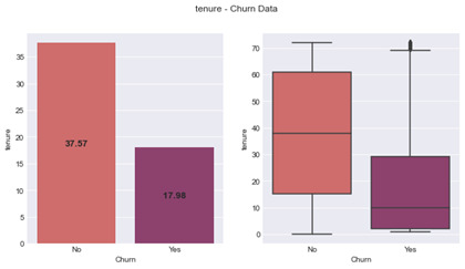
Figure 7: tenure – Churn Data

Multivariate analysis

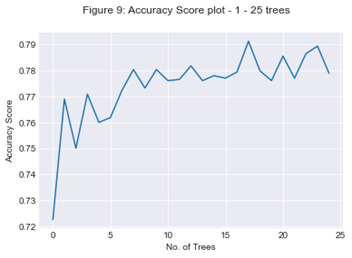
A random forest classifier model was devised for all attributes listed above to help determine the Churn response variable. The model was devised using the attributes listed in Figure 8 which also contains the feature importance ranked by the random forest classifier in order of highest to lowest. The number of trees in the model was then assessed to determine the optimum output of the model, evaluating the accuracy score from 1 to 25 trees. 17 trees presented an accuracy score of 79%.

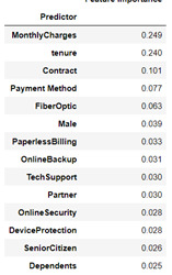
Figure 8: Feature Importance

[thepandas]

Capstone Project - Method

Sample

The Telco Customer Data was attained from Kaggle which was sourced from an IBM sample dataset. The data contains 7,043 individual customer records including customers who had churned within the last month – the creation date of the data was 24-02-2018. The Telco customer data was attained from those situated in the California area.

Measures

Response variable:

The response categorical variable Churn is a Yes/No indicator that shows in a customer has churned within the last month or not.

Predictor variables:

The predictor variables can be categorised by 3 different categories:

-        Demographic:

o   Gender – Categorical attribute stating the gender of the customer. This gets transformed to a numeric encoding.

o   Partner – An indicator to detail if the customer has a partner or not (Yes/No). This gets transformed to binary.

o   Dependents – Denotes if the customer has dependents or not (Yes/No). This gets transformed to binary.

o   Senior Citizen – classification on the customer being a senior citizen or not (Yes/No). This gets transformed to binary.

 -        Product/Services:

o   Fiber Optic – Indicator on the customer having Fiber Optic for their internet service. This attribute is derived from the internet service variable that has the responses DSL, Fiber Optic and No. This derived variable gets transformed to binary.

o   Tech Support – Indicator on the customer having tech support enabled as part of their services (Yes/No). This gets transformed to binary.  

o   Online Security – Indicator on the customer having Online Security enabled as part of their services (Yes/No). This gets transformed to binary.  

o   Online Backup – Indicator on the customer having Online Backup enabled as part of their services (Yes/No). This gets transformed to binary.  

o   Paperless Billing – Indicator on the customer having paperless Billing i.e. digital invoices or hard mail copies. This gets transformed to binary.  

o   Device Protection – indicator on the customer having device protection. This gets transformed to binary.

 -        Account Details:

o   Monthly Charges – the amount currently charged to the customer monthly.

o   Tenure – The number of months that a customer has stayed with the company.

o   Contract – Categorical variable defining the contract term the customer is on. This can be Monthly, One Year or Two Year. This gets transformed to a numeric encoding.

o   Payment Method Categorical variable defining the payment method for the account. This can include: ‘Electronic check’, ‘mailed check’, ‘bank transfer (automatic)’ and ‘Credit card (automatic)’. This gets transformed to a numeric encoding.

 Analyses

The initial exploratory analysis was conducted for all predictor variables. For this, frequency tables and graphs were produced for each categorical predictor variable to understand the count and distribution. Histograms were produced for quantitative data along with basic metrics such as mean, median and standard deviation to understand the spread.

When performing bivariate analysis between Churn (the response variable) and a categorical predictor variable, bar graphs were produced to show a visual representation of the data along with a Chi-Square test of independence to show the interaction between the two variables. The quantitative predictor variables were examined using a boxplot along with basic metrics such as mean, standard deviation, IQR and median. The Analysis of Variance (ANOVA) test was used to assess any associations between the predictor quantitative variables and the response variable.

A random forest classification model was produced to predict customers that were due to churn in the Telco Customer data. The model was devised on the training data that contained 70% of the data (n=4930) and testing was completed on the remaining 30% (n=2113). The model’s efficiency was determined by assessing the accuracy score based on the number of trees the model contained (assessing between 1 and 25 trees). A confusion matrix was produced, and the accuracy score was calculated for the effectiveness of the model on the test dataset.      

[thepandas]

Capstone Project - Introduction

The title of my project is: The association between the types of products/services a customer has and the likelihood of them churning based on the Telco Customer data. 

Based on the different services that Telco provide and are available (such as Phone Service, Multiple Lines, Internet Service, Online Security, Online Backup, Device Protection, streaming TV and Streaming Movies) I will be looking if there is any association in these customers churning. A generalised company view is that the more products/services a customer has the more ‘stickier’ the customer is and the less likely they are to churn. As a reporting analyst, I want to validate this hypothesis as these steps will be applicable to my company (I’m not using their data in the report due to data protection). This understanding will ultimately influence different areas within the company such as customer retention when creating proactive campaigns, this way we will be able to target specific customers with certain attributes.

The report itself will help from a generalisation perspective to create retention campaigns and for new products/packages. The limitation is that the reason why the customer churned is not known, there may be a false positive in the identification of accounts to target and ultimately the attribute to help identify the reason for churn may not be available in the current dataset.

[thepandas]

K-Means Cluster Analysis

Introduction

Throughout the course I have been looking at the association of alcohol dependence and alcohol consumption in relation to multiple explanatory variables (such as alcoholic parents) using the NESARC dataset. For this assignment I will be applying a k-means cluster model to 9 selected variables to represent the characteristics of the population. I ultimately be assessing these clusters and their normal alcohol consumption, trying to understand if there is a significant difference between them.

Data Management

The below code is for importing and cleaning the data prior to modelling.

# import libraries

import pandas as pd

import numpy as np

import matplotlib.pyplot as plt

from sklearn.model_selection import train_test_split

from sklearn import preprocessing

from sklearn.cluster import KMeans

 #import data

df = pd.read_csv(r'nesarc_pds.csv', low_memory=False, usecols=['S2AQ8B','S2AQ16B','S2AQ14','S1Q24FT','S1Q24IN','S1Q24LB'

                                                          ,'AGE','SEX','NUMPERS','S2DQ1','S2DQ2'])

 #rename columns

df.rename(columns={'S2AQ8B':'NoOfDrinks','S2AQ16B':'AgeDrinkOnceAWeek','S2AQ14':'NoYrsDrnkSame','S1Q24LB':'Weight',

                'S2DQ1':'FatherAlc','S2DQ2':'MotherAlc'}, inplace=True)

 # functions to calculate height

def heightInInches(feet, inches):

   if (feet != 99) & (inches != 99):

       return (feet * 12) + inches

   else:

       return np.nan

 # recode values

df['FatherAlc'] = df['FatherAlc'].map({1:1, 2:0, 9:np.nan})

df['MotherAlc'] = df['MotherAlc'].map({1:1, 2:0, 9:np.nan})

df['Male'] = df['SEX'].map({1:1, 2:0})

df['Weight'].replace(999, np.nan, inplace=True)

 # apply functions

df['Height'] = list(map(heightInInches, df['S1Q24FT'], df['S1Q24IN']))

 # cleanse 99 and blanks

cleanse_list = ['NoOfDrinks','AgeDrinkOnceAWeek','NoYrsDrnkSame']

 for col in cleanse_list:

   df[col] = df[col].replace('99', np.nan)

   df[col] = df[col].replace(r'^\s*$', np.nan, regex=True)

   df[col] = pd.to_numeric(df[col])

 cleansedData = df[['NUMPERS', 'AGE','Weight', 'NoOfDrinks','NoYrsDrnkSame', 'AgeDrinkOnceAWeek', 'FatherAlc', 'MotherAlc',

      'Height', 'Male']].copy()

 cleansedData.dropna(inplace=True)

 cleansedData.shape

 # standardise variables

variables = ['NUMPERS', 'AGE', 'Weight','NoYrsDrnkSame',

      'AgeDrinkOnceAWeek', 'FatherAlc', 'MotherAlc', 'Height', 'Male']

 cluster=cleansedData[variables].copy()

 for col in variables:

   cluster[col] = preprocessing.scale(cluster[col].astype('float64'))

 # split data into train and test

clus_train, clus_test = train_test_split(cluster, test_size=.3, random_state=123)

Cluster Model

# creating a cluster analysis for 1 -9 clusters

from scipy.spatial.distance import cdist

clusters=range(1,10)

mean_dist=[]

 # iterate over 1 -9 clusters to assess suitable number

for k in clusters:

   model=KMeans(n_clusters=k)

   model.fit(clus_train)

   clus_assign=model.predict(clus_train)

  mean_dist.append(sum(np.min(cdist(clus_train, model.cluster_centers_, 'euclidean'), axis=1))

                   / clus_train.shape[0])

 # plot the average distance from the observations from the cluster centroids

plt.plot(clusters, mean_dist)

plt.xlabel('Number of Clusters')

plt.ylabel('average distance')

plt.title('Selectingk with the Elbow Method')

# looking at 2 clusters, where the model starts to level off

model2=KMeans(n_clusters=2)

model2.fit(clus_train)

clusassign=model2.predict(clus_train)

Canonical Discriminant Analysis

# use PCA - canonical discirminant analysis as reduction technique

from sklearn.decomposition import PCA

pca_2 = PCA(2)

plot_columns = pca_2.fit_transform(clus_train)

plt.scatter(x=plot_columns[:,0], y=plot_columns[:,1], c=model2.labels_,)

plt.xlabel('Canonical Variable 1')

plt.ylabel('Canonical Variable 2')

plt.title('Scatterplot of Canonical Variables for 2 clusters')

plt.show()

Cluster metrics & ANOVA

# understanding the clusters

clus_train.reset_index(level=0, inplace=True)

 cluslist=list(clus_train['index'])

 labels=list(model2.labels_)

 newlist=dict(zip(cluslist, labels))

 newclus=pd.DataFrame.from_dict(newlist, orient='index')

 newclus.columns = ['cluster']

 newclus.reset_index(level=0, inplace=True)

 merged_train=pd.merge(clus_train, newclus, on='index')

 merged_train.cluster.value_counts()

clustergrp = merged_train.groupby('cluster').mean()

print(clustergrp)

# comparing the number of drinks an individual usually drinks between the two groups

 NoOfDrinksData = cleansedData['NoOfDrinks']

 drnks_train, drnks_test = train_test_split(NoOfDrinksData, test_size=.3, random_state=123)

drnks_train1=pd.DataFrame(drnks_train)

drnks_train1.reset_index(level=0, inplace=True)

merged_train_all=pd.merge(drnks_train1, merged_train, on='index')

sub1 = merged_train_all[['NoOfDrinks','cluster']].dropna()

 import statsmodels.formula.api as smf

import statsmodels.stats.multicomp as multi

 drnksmod = smf.ols(formula='NoOfDrinks ~ C(cluster)', data=sub1).fit()

print(drnksmod.summary())

print('Avg No of Drinks by cluster')

print(sub1.groupby('cluster')['NoOfDrinks'].mean())

print('\n Std Dev No of Drinks by cluster')

print(sub1.groupby('cluster')['NoOfDrinks'].std())

Summary

A k-means cluster model was applied to the NESARC dataset for those that consume alcohol and returned all valid responses to the 10 variables. The 9 variables that were used for the model contained 3 binary variables (Father Alcoholic, Mother Alcoholic and Male) and 6 quantitative variables (Number of persons in household, Age, Weight, Height, Number of years drinking the same as currently do and Age drinking Once a week).

As the optimum number of clusters was unknown, the model was applied using clusters 1 – 9 to understand the most effective model. A plot was produced (as shown in the ‘Cluster Model’ section, titled: 'Selectingk with the Elbow Method'), detailing the number of clusters and the average distance – using the elbow method to determine when the average distance was levelling off, I subjectively selected points 2 and 6 for the number of clusters. Further analysis was conducted on the 2-cluster model.

 Canonical discriminant analysis was applied to the 2-cluster model to reduce the number of variables to 2 in which the variables account for the variance in the original 9 variables. The 2 clusters (see scatter plot above in Canonical Discriminant Analysis section) take distinct sides however there is a considerable amount of overlap meaning there is no good separation between the clusters. The clusters are not completely dense, resulting in the variance being higher and less correlated with each other.  

 From the means of the cluster variables, I was able to determine the following for the 2 groups:

-        Cluster 0:

o   Predominately Female.

o   More likely than cluster 1 to have an alcoholic parent.

o   More likely than cluster 1 to start drinking at least once a week at an earlier age.

-        Cluster 1:

o   Predominately Male.

o   Have been drinking current alcohol consumption for a longer period than cluster 0.

o   Tend to be living with less people than cluster 0.

To assess the 2 clusters in association with alcohol consumption, an Analysis of Variance model was applied to determine if the was a significant difference between the two groups and the number of alcoholic drinks an individual normally consumes when drinking. Those in cluster 0 had a mean number of drinks consumed as 2.0 with a standard deviation of 1.7. Those in cluster 1 had a mean number of drinks consumed as 3.1 with a standard deviation of 2.8. The F-statistic was 758.0 with a p-value of <0.001 suggesting the two groups were significantly different in relation to alcohol consumption.  

[thepandas]

LASSO Regression Model - LARs

Introduction

Throughout the course I have been looking at the association of alcohol dependence in relation to many variables but mainly focusing on alcoholic parents using the NESARC dataset. For this assignment I will be applying a LASSO Regression model to determine alcohol consumption based on general profile characteristics/backgrounds.  

Data Management

#import libraries

import pandas as pd

import numpy as np

import matplotlib.pyplot as plt

from sklearn.model_selection import train_test_split

from sklearn.linear_model import LassoLarsCV

from sklearn import preprocessing

 #import data

df = pd.read_csv(r'nesarc_pds.csv', low_memory=False, usecols=['S2AQ8B','S2AQ16B','S2AQ14','S3AQ2A1','S3BQ1A5','S3BQ1A6',

                                                              'BUILDTYP','NUMPERS','AGE','SEX','S1Q1C','S1Q1D1','S1Q1D2',

                                                              'S1Q1D3','S1Q1D4','S1Q1D5','S1Q6A','S1Q10A','S1Q24FT','S1Q24IN',

                                                            'S1Q24LB'])

 #height in inches function

def HeightInInches(Feet, inches):

   return (Feet * 12) + inches

 #apply functions and recording

df['Height'] = list(map(HeightInInches, df['S1Q24FT'], df['S1Q24IN']))

# recode sex

df['Male'] = df['SEX'].map({1:1, 2:0})

 recordYesNo = ['S1Q1C','S1Q1D1','S1Q1D2','S1Q1D3','S1Q1D4','S1Q1D5']

 for field in recordYesNo:

   df[field] = df[field].map({1:1, 2:0})

 #cleanse numeric fields – replacing nan in blank fields.

numeric_cols = ['S2AQ8B','S2AQ14','S2AQ16B']

 for col in numeric_cols:

   df[col] = df[col].replace('^\s*$', np.nan, regex=True)

   df[col] = pd.to_numeric(df[col])

 #rename fields

df.rename(columns={'S1Q1C':'HisOrLat','S1Q1D1':'AmInd','S1Q1D2':'Asian','S1Q1D3':'BlackAfAm','S1Q1D4':'HawOrPacific','S1Q1D5':'Whi','S1Q6A':'HighestEd','S1Q10A':'Income','S1Q24LB':'Income','S2AQ8B':'DrinksUsualCon','S2AQ14':'YrsDrnkSame','S2AQ16B':'AgeDrnkOnceWeek','S3BQ1A5':'Cannab','S3BQ1A6':'Coca'}, inplace=True)

 # drop nans

df2 = df[['BUILDTYP', 'NUMPERS', 'AGE', 'SEX', 'HisOrLat', 'AmInd', 'Asian','BlackAfAm', 'HawOrPacific', 'Whi', 'HighestEd'

         ,'Income','Income', 'DrinksUsualCon', 'YrsDrnkSame', 'AgeDrnkOnceWeek','Cannab', 'Coca', 'Height', 'Male']].copy()

 df2.dropna(inplace=True)

 # divide data into predictors and target and scale predictors.

 pred_cols = ['BUILDTYP', 'NUMPERS', 'AGE', 'SEX', 'HisOrLat', 'AmInd', 'Asian','BlackAfAm', 'HawOrPacific', 'Whi', 'HighestEd','Income','Income','YrsDrnkSame', 'AgeDrnkOnceWeek','Cannab', 'Coca', 'Height', 'Male']

 predictors = df2[pred_cols].copy()

 for col in pred_cols:

   predictors[col] = preprocessing.scale(predictors[col].astype('float64'))

 target = df2['DrinksUsualCon']

 pred_train, pred_test, tar_train, tar_test = train_test_split(predictors, target, test_size=.3, random_state=123)

 Lasso Regression Model

 # lasso regression model - using 10 fold

model=LassoLarsCV(cv=10, precompute=False).fit(pred_train, tar_train)

dict(zip(predictors.columns, model.coef_))

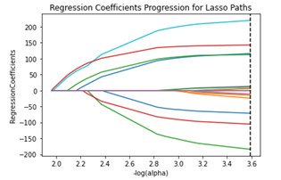
# plot coefficient progression

 m_log_alphas = -np.log10(model.alphas_)

ax = plt.gca()

plt.plot(m_log_alphas, model.coef_path_.T)

plt.axvline(-np.log10(model.alpha_), linestyle='--', color='k', label='alpha CV')

 plt.ylabel('RegressionCoefficients')

plt.xlabel('-log(alpha)')

plt.title('Regression Coefficients Progression for Lasso Paths')

Measurables

 # plot mean square error for each fold

m_log_alphascv = -np.log10(model.cv_alphas_)

plt.figure()

plt.plot(m_log_alphascv, model.mse_path_, ':')

plt.plot(m_log_alphascv, model.mse_path_.mean(axis=-1), color='k', label='Average Across the folds', linewidth=2)

plt.axvline(-np.log10(model.alpha_), linestyle='--', color='k', label='alpha CV')

 plt.legend()

plt.xlabel('-log(alpha)')

plt.ylabel('Mean squared error')

plt.title('Mean squared error on each fold')

# MSE from training and test data

from sklearn.metrics import mean_squared_error

 train_error = mean_squared_error(tar_train, model.predict(pred_train))

test_error = mean_squared_error(tar_test, model.predict(pred_test))

 print('Training data MSE')

print(train_error)

print('Test data MSE')

print(test_error)

rsquared_train = model.score(pred_train, tar_train)

rsquared_test = model.score(pred_test, tar_test)

 print('Training data r-squared')

print(rsquared_train)

print('Test data r-squared')

print(rsquared_test)

Summary

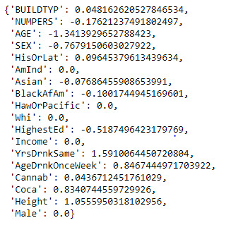
The LASSO regression model was constructed to determine the number of drinks normally consumed on days when an individual drinks alcohol. The model used 17 explanatory variables (consisting of categorical and quantitative variables), had a train test split of 70:30 and used 10 folds for the cross-validation strategy. Of the 17 variables only 12 were retained by the model. The top 4 explanatory variables with the largest coefficients and association with number of drinks normally consumed were: Years Drank the same (1.59), Age (-1.34), Height (1.06) and Age Drinking Once a Week (0.85).  

 The mean squared error on each fold followed the same pattern however have a large variability as you can see from the plot produced. This is most likely due to the large number of samples where the data subsets are not consistent with the type of samples. The test data had a lower mean square error score at 65.8 in comparison to the training data at 85.5. The r-squared values were 8% and 9% respectively for training and test datasets suggesting that the explanatory variables can only account for a small portion of the variance in the response variable. Additional variables would be required to provide any form of accuracy in predicting the number of drinks usual consumed by an individual.  

[thepandas]

Random Forest Model

The topic I am looking at is the association of alcoholic parent(s) and the child becoming alcohol dependent using the NESARC dataset. For this assignment I will be constructing a Random Forest Model to determine alcohol dependence.

Data Management

# import libraries import pandas as pd import numpy as np import matplotlib.pyplot as plt from sklearn.model_selection import train_test_split from sklearn.tree import DecisionTreeClassifier from sklearn.metrics import classification_report import sklearn.metrics # feature importance from sklearn import datasets from sklearn.ensemble import ExtraTreesClassifier from sklearn.ensemble import RandomForestClassifier

# read filtered file in df = pd.read_csv('nesarc_ml_rf.csv', low_memory=False, usecols=['S2DQ1','S2DQ2','S2BQ2D','S2AQ16B','SEX','AGE','S1Q24LB'])

print(df.shape)

# derive variables: Alcohol Dependent, Alcoholic Parents def alcParent(father, mother):    if (father == 1) | (mother == 1):        return 1    else:        return 0

def alcDependence(age):    if (age.isnumeric()) & (age != 99):        return 1    else:        return 0

df['AlcParent'] = list(map(alcParent, df['S2DQ1'], df['S2DQ2'])) df['AlcDep'] = list(map(alcDependence, df['S2BQ2D'])) df['MaleGender'] = df['SEX'].map({2:0, 1:1})

#renaming df.rename(columns={'S2AQ16B':'AgeDrinkOnceWeek', 'S1Q24LB': 'Weight_lbs'}, inplace=True)

# numeric formating numeric_cols = ['AGE','MaleGender', 'AgeDrinkOnceWeek','Weight_lbs']

for colname in numeric_cols:    df[colname] = df[colname].replace(r'^\s*$', np.nan, regex=True)    df[colname] = pd.to_numeric(df[colname])

#drop nan records df.dropna(inplace=True)

Model Generation

# split data for train and testing

predictors = df[['AGE','MaleGender','Weight_lbs','AgeDrinkOnceWeek','AlcParent']] targets = df['AlcDep']

x_train, x_test, y_train, y_test = train_test_split(predictors, targets, test_size=0.3)

print(x_train.shape) print(y_train.shape) print(x_test.shape) print(y_test.shape)

# build random forest model classifier =RandomForestClassifier(n_estimators=25) classifier=classifier.fit(x_train, y_train)

predictions=classifier.predict(x_test)

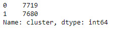
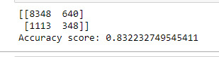
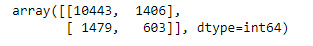
print(sklearn.metrics.confusion_matrix(y_test, predictions)) print('Accuracy score: {}'.format(sklearn.metrics.accuracy_score(y_test, predictions)))

# fit Extra Trees model to the data model = ExtraTreesClassifier() model.fit(x_train, y_train) # display feature importance scores print(predictors.columns) print(model.feature_importances_)

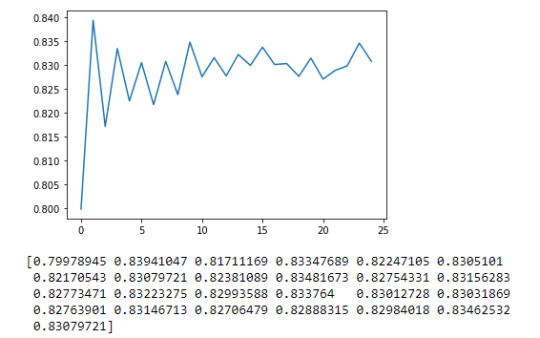
# determine prediction efficiency based on the number of trees trees=range(25) accuracy=np.zeros(25)

for idx in range(len(trees)):    classifier2 = RandomForestClassifier(n_estimators=idx+1)    classifier2 = classifier2.fit(x_train, y_train)    prediction2 = classifier2.predict(x_test)    accuracy[idx] = sklearn.metrics.accuracy_score(y_test, prediction2)

plt.cla() plt.plot(trees,accuracy) plt.show() print(accuracy)

Summary

The Random Forest Model analysis was performed to determine the alcohol dependence categorical variable. The model used Age, Gender, Weight, Age Drinking Once a Week and Alcoholic Parents indicator. The model was created using a 70:30 split for train and test data. The feature importance scores returned Weight and Age Drinking Once a Week as the highest contributing attributes at 0.404 and 0.285 respectively.

The Random Forest accuracy was 83.2% on a 25 estimators/trees model. When analyzing the estimators (as seen in the graph above), a 1 tree estimator was more efficient and accurate at 83.9% and therefore more appropriate for the current model.    

[thepandas]

Classification Tree

The topic I am looking at is the association of alcoholic parent(s) and the child becoming alcohol dependent using the NESARC dataset. For this assignment I will be constructing a Classification Tree to determine alcohol dependence.

Data Management

import pandas as pd

import numpy as np

from sklearn.model_selection import train_test_split

from sklearn.tree import DecisionTreeClassifier

from sklearn.metrics import classification_report

import sklearn

 pd.set_option('display.max_columns', 100)

 # data import

df = pd.read_csv(r'nesarc_pds.csv', low_memory=False,

                usecols=['S2DQ1','S2DQ2','S2BQ2D','S2AQ16B','SEX','AGE','S1Q24LB'])

# S2DQ1 - Father Alcoholic

# S2DQ2 - Mother Alcoholic

# S2BQ2D = Age at onset alcohol Dependence

# S2AQ16B = Age when started drink at least once a week

# SEX - 1 male, 2 Female

# AGE - 18 - 97 age 98 = 98 or older

# S1Q24LB - weight in pounds

 # Alc dependent, Alc Parent functions

def alcParent(father, mother):

   if (father == 1) | (mother == 1):

       return 1

   else:

       return 0

     def alcDependence(age):

   if (age.isnumeric()) & (age != 99):

       return 1

   else:

       return 0

  # apply functions/recoding

df['AlcParent'] = list(map(alcParent, df['S2DQ1'], df['S2DQ2']))

df['AlcDep'] = list(map(alcDependence, df['S2BQ2D']))

df['MaleGender'] = df['SEX'].map({2:0, 1:1})

  #renaming /formatting

df.rename(columns={'S2AQ16B':'AgeDrinkOnceWeek', 'S1Q24LB': 'Weight_lbs'}, inplace=True)

 numeric_cols = ['AGE','MaleGender', 'AgeDrinkOnceWeek','Weight_lbs']

 for colname in numeric_cols:

   df[colname] = df[colname].replace(r'^\s*$', np.nan, regex=True)

   df[colname] = pd.to_numeric(df[colname])

 df.dropna(inplace=True)

  Decision Tree Classifier

predictors = df[['AGE','MaleGender','Weight_lbs','AgeDrinkOnceWeek','AlcParent']]

targets = df[['AlcDep']]

x_train, x_test, y_train, y_test = train_test_split(predictors, targets, test_size=0.4)

 classifier=DecisionTreeClassifier()

classifier=classifier.fit(x_train,y_train)

 predictions=classifier.predict(x_test)

 sklearn.metrics.confusion_matrix(y_test, predictions)

sklearn.metrics.accuracy_score(y_test, predictions)

Summary

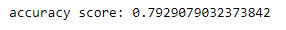
 The purpose of this model was to determine when a respondent was alcohol dependent, where the variable Age at Onset Alcohol Dependence was used to derive a binary response variable. The model uterlised 5 features in total and produced an accuracy score of 79.3%. Ideally additional features would be added to the model to increase the accuracy score.  

[thepandas]

Regression Modelling in Practice – Week 4 - Logistic Regression

The topic I am looking at is the association of alcoholic parent(s) and the child becoming alcohol dependent using the NESARC dataset. My hypothesis is that those respondents who have alcoholic parents are more likely to then become alcohol dependent.

For my analysis, this week I will be using the following variables:

-       AGE

-       SEX

-       S2DQ1 – Alcoholic Father

-       S2DQ2 – Alcoholic Mother

-       S2BQ2D – Age at onset Alcohol Dependence

-       S2AQ16B – Age when started drinking at least once a week.

Data Management

Below are the data management decisions made for the logistic regression model along with the code.

import pandas as pd

import numpy as np

import statsmodels.formula.api as smf

import statsmodels.api as sm

 pd.set_option('display.max_columns', 100)

 df = pd.read_csv('nesarc_pds.csv', low_memory=False, usecols=['S2DQ1','S2DQ2','S2BQ2D','S2AQ16B','SEX','AGE'])

 # fucntions to derive categorical data points

def alcParent(Farther, Mother):

   if (Farther == 1) | (Mother == 1):

       return 1

   else:

       return 0

  def alcDependence(value):

   if (value.isnumeric()) & (value != 99):

       return 1

   else:

       return 0

     def DrinkingBefore18(Age):

   if (Age > 0) & (Age < 18):

       return 1

   else:

       return 0

    def maleRes(Gender):

   if Gender == 1:

       return 1

   elif Gender == 2:

       return 0

 # convert fields to numeric

numeric_cols = ['AGE','S2AQ16B']

 for attribute in numeric_cols:

   df[attribute] = df[attribute].replace(r'^\s*$', np.nan, regex=True)

   df[attribute] = pd.to_numeric(df[attribute])

 # apply functions

df['AlcoholicParent'] = list(map(alcParent, df['S2DQ1'], df['S2DQ2']))

df['AlcDep'] = list(map(alcDependence, df['S2BQ2D']))

df['MaleResp'] = list(map(maleRes, df['SEX']))

df['drnkBefore18'] = list(map(DrinkingBefore18, df['S2AQ16B']))

 Logistic Regression Model

log_reg = smf.logit(formula='AlcDep ~ AlcoholicParent + MaleResp + drnkBefore18', data=df).fit()

print(log_reg.summary())

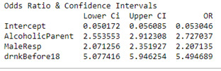
print('Odds Ratio & Confidence Intervals')

params = log_reg.params

conf = log_reg.conf_int()

conf['Odds Ratio'] = params

conf.columns = ['Lower Ci','Upper CI', 'OR']

print(np.exp(conf))

Summary

From the logistic regression model produced in this analysis, no confounding variables were identified when iteratively adding variables to the model. Based on the sample from the NESARC dataset, the hypothesis stated in the introduction can be accepted as those with alcoholic parent(s) were 2.7 more times likely to be alcohol dependent than those who did not have alcoholic parents (OR=2.7, 95% CI=2.6 – 2.9, p<0.001). Respondents who started drinking at least once a week prior to the age of 18 were also 5.5 more times likely to be alcohol dependent than those who started drinking once a week after the age of 18 (OR= 5.5, 95% CI = 5.1 – 5.9, p <0.001). Finally, Male respondents were also 2.2 times more likely to be alcohol dependent than females (OR=2.2m 95% CI = 2.1 – 2.4, p< 0.001).

[thepandas]

Multiple Regression Model

Introduction

The analysis thus far has focused on the association of alcoholic parent(s) and the child becoming alcohol dependent using the NESARC dataset. For this week’s topic I will be altering my focus to include quantitative variables by assessing the age an individual is alcohol dependent using various explanatory variables within the dataset. Primary assessing if there is an association between the age someone starts drinking to the age of alcohol dependence for those who have/had alcoholic parent(s).

Data Management

# import libraries

import pandas as pd

import numpy as np

import matplotlib.pyplot as plt

import seaborn as sns

import statsmodels.api as sm

import statsmodels.formula.api as smf

 # read in data

df = pd.read_csv('nesarc_pds.csv', low_memory=False, usecols=['S2AQ8A','S2AQ14','S2AQ16A','S2AQ16B','S2BQ2D','S2DQ1','S2DQ2'])

 # create functions to derive binary indicators

def alcParent(Father, Mother):

   if (Father ==1) | (Mother == 1):

       return 1

   else:

       return 0

  def alcDependence(age):

   if (age.isnumeric()) & (age != 99):

       return 1

   else:

       return 0

 # Apply functions to data

df['AlcParent'] = list(map(alcParent, df['S2DQ1'], df['S2DQ2']))

df['AlcDep'] = list(map(alcDependence, df['S2BQ2D']))

 # cleanse numeric fields

Numeric_fields = ['S2AQ8A','S2AQ14','S2AQ16A','S2AQ16B','S2BQ2D']

 for field_name in Numeric_fields:

   df[field_name] = df[field_name].replace(r'^\s*$', np.nan, regex=True)

   df[field_name] = pd.to_numeric(df[field_name])

 # recode frequency for alcohol frequency

df['AlcConFrequency'] = df['S2AQ8A'].map({1:365, 2:286, 3:182, 4:104, 5:52,6:30, 7:12, 8:9, 9:5, 10:2, 99:99})

 #subset of data to remove invalid options and only return those who are alc dependent

df.rename(columns={'S2AQ14':'YrsDrinkingSameAsLast12Mths', 'S2AQ16A':'AgeWhenStartedDrinking', 'S2AQ16B':'AgeDrinkingOnceAWeek',

                  'S2BQ2D':'AgeAtAlcDep'}

         , inplace=True)

 # Get those that are alcohol dependent and have alc parents

df2 = df.loc[(df['AlcParent'] == 1) & (df['AlcDep'] == 1) & (df['YrsDrinkingSameAsLast12Mths'] != 99) & (df['AlcConFrequency'] != 99) &

            (df['AgeWhenStartedDrinking'] < 99) & (df['AgeDrinkingOnceAWeek'] < 99) & (df['AgeAtAlcDep'] < 99)]

df2.dropna()

 # centre variables

df2['YrsDrinkingSameAsLast12Mths_c'] = df2['YrsDrinkingSameAsLast12Mths'] - df2['YrsDrinkingSameAsLast12Mths'].mean()

df2['AgeWhenStartedDrinking_c'] = df2['AgeWhenStartedDrinking'] - df2['AgeWhenStartedDrinking'].mean()

df2['AgeDrinkingOnceAWeek_c'] = df2['AgeDrinkingOnceAWeek'] - df2['AgeDrinkingOnceAWeek'].mean()

df2['AlcConFrequency_c'] = df2['AlcConFrequency'] - df2['AlcConFrequency'].mean()

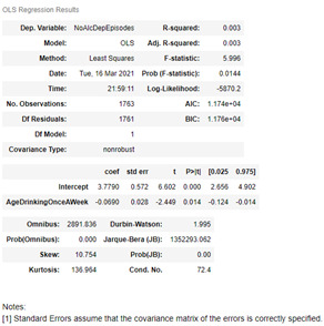
  Results summary

reg1 = smf.ols('AgeAtAlcDep ~ AlcConFrequency_c + AgeDrinkingOnceAWeek_c + AgeWhenStartedDrinking_c + YrsDrinkingSameAsLast12Mths_c', data=df2).fit()

print(reg1.summary())

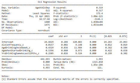
The model primary focused on the association of the age at alcohol dependence and the age when started drinking, which was positively correlated (Beta  =0.5396, p= <0.001). Additional variables were added to the model to improve the fit, including positive associations between age of alcohol dependence and Alcohol Consumption Frequency (Beta= 0.0157, p=<0.001); Age Drinking Once a week (Beta=0.4329, p=<0.001) and Years drinking the same volume as the last 12 months (Beta=0.2505, p=<0.0001). The model displayed a small R-Squared, meaning that only 32% of the response variable variability could be explained by the explanatory variables. This suggests the model is not sufficient and would require additional explanatory variables to improve the fit.

 Regression Diagnostic plots

# check to see if residuals are normally distributed

fig1 = sm.qqplot(reg1.resid, line='r')

The q-q plot above illustrates the variability in the model and that the residuals are not normally distributed within the upper and lower quantiles.  

 stdres=pd.DataFrame(reg1.resid_pearson)

fig2=plt.plot(stdres, 'o', ls='None')

plt.show()

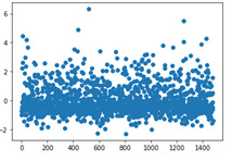
The standardized residuals plot for all observations also displays that a large number of the residuals are outside 2 standard deviations, meaning the level of error in the model is poor and that other key explanatory variables should be included within the model. It also suggests that there may be some outliers within the data, especially with those close to 3-6 deviations from the mean.

 Alc Con Frequency

fig3 = plt.figure(figsize=(12,8))

fig3 = sm.graphics.plot_regress_exog(reg1, 'AlcConFrequency_c', fig=fig3 )

The output above displays the additional diagnostic plots for the Alcohol Consumption Frequency explanatory variable. The ‘Residual versus AlcConFrequency_c’ plot shows the residuals for the values of Alcohol Consumption Frequency; these appear to be evenly distributed at each given frequency. Each frequency also displays a wide variability in the residuals meaning the fit to this variable appears to be unpredictable based on this Alcohol Consumption Frequency. The Partial regression plot looks at the effect of the Alcohol Consumption Frequency variable given the other explanatory variables exist within the model. By controlling for this we can determine if there is a non-linear association that should be considered in the model. For this plot, the residuals are spread out in a random pattern around the partial regression line suggesting there is no obvious non-linear regression.    

 Age Drinking Once a Week

fig3 = plt.figure(figsize=(12,8))

fig3 = sm.graphics.plot_regress_exog(reg1, 'AgeDrinkingOnceAWeek_c', fig=fig3 )

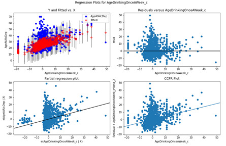
The Residuals versus AgeDrinkingOnceAWeek_c plot suggests there could be a non-linear relationship based on the residuals towards 20 – 40 although the bulk of the residuals are centered around 0. The Partial regression plot displays the AgeDrinkOnceAWeek_c variable while controlling for the other variables and perceivably a random set of residuals around -5 – 10. A non-linear pattern could be applied but would only marginally increase the fit of the model.

Age When Started Drinking

fig4 = plt.figure(figsize=(12,8))

fig4 = sm.graphics.plot_regress_exog(reg1, 'AgeWhenStartedDrinking_c', fig=fig4 )

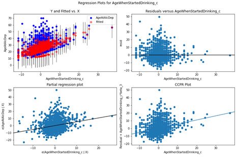
Based on the Residual and partial regression plot for the AgeWhenStartedDrinking_c variable, there is no non-linear relationship, and the residuals are primarily centered around the mean with a wide dispersion.

 Years Drinking same as last 12 months

fig5 = plt.figure(figsize=(12,8))

fig5 = sm.graphics.plot_regress_exog(reg1, 'YrsDrinkingSameAsLast12Mths_c', fig=fig5 )

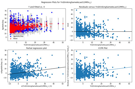
Based on the Residuals and Partial regression plot, the YrsDrinkingSameAsLast12Mths_c variable looks like it could marginally increase fit with a non-linear regression element however due to the dispersion the benefits will be marginal.  

 #Leverage Plot

Fig8 = sm.graphics.influence_plot(reg1, size=1)

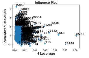
The leverage plot displays the outliers that were shown in the standardized residual plot and noticeably the leverage that these outliers have individually are minimal however due to the number that are outside 2.5 standard deviations of the mean, the impact will become more apparent.

 Summary

In summary the model included explanatory variables that had a correlation with the Age of Alcohol Dependence variable however the fit (r-squared) was only 32%. When observing the individual diagnostic plots it was obvious that the residuals for each variable were deviating largely from the response variable. Additional key explanatory variables would be required to improve the fit of this model.

[thepandas]

Basic Linear Regression

The topic I am looking at is the association of alcoholic parent(s) and the child becoming alcohol dependent using the NESARC dataset. For this week’s topic I’ll be altering my focus to include quantitative variables by assessing if there is an association between the age an individual starts drinking once a week to the number of alcoholic dependent episodes for those who have alcoholic parents. For this examination I will be using the following variables from the NESARC dataset.

-        AGE WHEN STARTED DRINKING AT LEAST ONCE A WEEK

-        NUMBER OF EPISODES OF ALCOHOL DEPENDENCE

-        BLOOD/NATURAL FATHER EVER AN ALCOHOLIC OR PROBLEM DRINKER

-        BLOOD/NATURAL MOTHER EVER AN ALCOHOLIC OR PROBLEM DRINKER

 Data Management

# import libraries

import pandas as pd

import numpy as np

import seaborn as sns

import statsmodels.formula.api as smf

import matplotlib.pyplot as plt

import scipy

 df = pd.read_csv(r'nesarc_data_reg.csv', usecols=[‘S2AQ16B’,’ S2BQ2E’, 'S2DQ1','S2DQ2'] low_memory=False, index_col=0)

print(df.shape)

 # alc parent function

def AlcParent(Father, Mother):

   if (Father == 1) | (Mother == 1):

       return 1

   else:

       return 0

  # cleanse numeric fields

NumericCols = ['S2AQ16B','S2BQ2E']

 for columnName in NumericCols:

   df[columnName] = df[columnName].replace(r'^/s+$', np.nan, regex=True)

   df[columnName] = df[columnName].replace(' ',np.nan)

   df[columnName] = pd.to_numeric(df[columnName])

 # rename column names

df.rename(columns= {'S2AQ16B':'AgeDrinkingOnceAWeek', 'S2DQ1':'FatherAlc', 'S2DQ2':'MotherAlc', 'S2BQ2E':'NoAlcDepEpisodes'}, inplace=True)

 # derive new variable for either parent being an alcoholic

df['AlcParent'] = list(map(AlcParent, df['FatherAlc'], df['MotherAlc']))

print(df.head())

 # create subset of data removing nulls and invalid values as per codebook

sub1 = df.loc[(df['AgeDrinkingOnceAWeek'] > 3) & (df['AgeDrinkingOnceAWeek'] < 92) & (df['NoAlcDepEpisodes'] <= 98 ) &

             (df['AlcParent'] == 1 ), ['AgeDrinkingOnceAWeek','NoAlcDepEpisodes']]

 sub1.dropna()

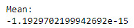
  Centering

sub1['AgeDrinkingOnceAWeekCentering'] = sub1['AgeDrinkingOnceAWeek'] - sub1['AgeDrinkingOnceAWeek'].mean()

 print('Mean:')

print(sub1['AgeDrinkingOnceAWeekCentering'].mean())

 print('Value Counts:')

print(sub1['AgeDrinkingOnceAWeekCentering'].value_counts())

 sns.displot(sub1['AgeDrinkingOnceAWeekCentering'].dropna(), kind='hist')

plt.show()

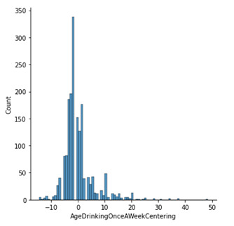
By displaying the frequency table in a histogram we can see that the data is centred around zero, with a right skew due to age parameters.

Linear Regression Model

sns.regplot(x='AgeDrinkingOnceAWeek', y='NoAlcDepEpisodes', data=sub1)

plt.show()

 print('Pearson Correlation coefficient {}'.format(scipy.stats.pearsonr(sub1['AgeDrinkingOnceAWeek'],sub1['NoAlcDepEpisodes'])))

 reg = smf.ols(formula='NoAlcDepEpisodes ~ AgeDrinkingOnceAWeek', data=sub1).fit()

reg.summary()

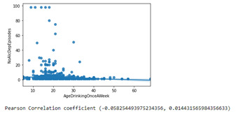
Summary

 The results from the linear regression model show that there was no association between the age an individual starts drinking once a week to the number of alcoholic dependent episode for those with alcoholic parents. The Pearson correlation coefficient was -0.058 (p-value 0.014) resulting in little to no relationship with the formula being ŷ = 3.78 – 0.069x. The model also exhibits a small R-Squared value, 0.003, meaning that the proportion of the variance in the response variable that can be explained by the explanatory variable is extremely small.

[thepandas]

About the NESARC data

Sample

The data used in my analysis so far is from the first wave of the National Epidemiologic Survey on Alcohol and Related Conditions (NESARC) data which was the largest ever comorbidity study of multiple mental health disorders among US adults, including alcohol and other substances use disorders, personality disorders, and anxiety and mood disorders. The survey was conducted in 2001-2002 with interviews of a total sample size of 43,093. It is stated that Blacks, Hispanics and adults aged 18-24 years were oversampled in this data. The sample was adjusted accordingly to the US population based on the 2000 Decennial Census. For my analysis, all data was used except for those where the answer was unknown. 

Data Collection procedure

The data collection for the NESARC survey was conducted via face-to-face interviews for each of the respondents in 2001 - 2002. These respondents who were 18 or older were required to answer observational questions around the selected topics. The collection enabled a diverse gathering of data by distinct groups selected by state and key sociodemographic characteristics again in line with the census defined variables. The data was validated by randomly selected call backs to respondents, checking that a subset of their answers matched their original responses.

Measures

The 3 measures that I derived or analysed within my data analysis so far were all taken from the NESARC dataset. This enabled analysis on the association of alcoholic parent(s) and the child becoming alcohol dependent, using the variables:

-        Alcoholic Parent(s) – I derive this from Mother Alcoholic and Father Alcoholic variables within the NESARC dataset. If either of these parents are alcoholic, I set this variable to True, else False. If the participants response was unknown this variable is also set to False. This was used as an explanatory variable. 

-        Alcohol Dependence – this is derived from the variable ‘Age at Onset of Alcohol Dependence’. This only includes those that knew the year of onset alcohol dependence and did not include the 90 respondents where the answer was unknown. This was used as an response variable.

-        Age When Started Drinking – simple taken from the NESARC survey ‘Age when started Drinking, not counting small tastes or sips’ which ranged from 5 – 83 years old. This was used as an explanatory variable.

[thepandas]

Statistical Interaction

The topic I am looking at is the association of alcoholic parent(s) and the child becoming alcohol dependent using the NESARC dataset. The statistical interaction that I will be testing is the age a respondent starts drinking. This moderator categorical variable will comprise of those who started drinking under the age of 21, over the age of 21 and those who did not respond or was unknown.

 Data Management

Import libraries and data as per prior modules. The only addition for this week’s project is the ageCategory function.

# import libraries and data

import pandas as pd

import numpy as np

import seaborn as sns

import matplotlib.pyplot as plt

import scipy

 pd.set_option('display.max_columns',100)

pd.set_option('display.max_rows',100)

 df = pd.read_csv(r'nesarc_pds.csv', low_memory=False, usecols=['S2AQ16A','S2BQ2D','S2DQ1','S2DQ2'])

 df.rename(columns={'S2DQ1':'Father_Alcoholic', 'S2DQ2':'Mother_Alcoholic', 'S2AQ16A':'AgeStartedDrinking',

              'S2BQ2D':'AgeAlcoholDependence'}, inplace=True)

 # functions to derive new variables

def alcParent(Father, Mother):

   if (Father ==1)|(Mother == 1):

       return 1

   else:

       return 0

    def alcDependence(value):

   if (value.isnumeric()) and (value != 99):

       return 1

   elif value == 99:

       return np.nan

   else:

       return 0

     def ageCategory(age):

   if (age >= 21) and (age != 99):

       return '21 and older'

   elif (age < 21) and (age != 99):

       return '20 and younger'

   else:

       return np.nan

  # clean age started drinking data

df['AgeStartedDrinking'].replace('^/s+$', np.nan, inplace=True, regex=True)

df['AgeStartedDrinking'] = pd.to_numeric(df['AgeStartedDrinking'], errors='coerce')

 # apply functions

df['AlcParent'] = list(map(alcParent, df['Father_Alcoholic'], df['Mother_Alcoholic']))

df['AlcDependence'] = list(map(alcDependence, df['AgeAlcoholDependence']))

df['AgeStartedCat'] = list(map(ageCategory, df['AgeStartedDrinking']))

 # set data types as category

df['AlcParent'].astype('category')

df['AlcDependence'].astype('category')

df['AgeStartedCat'].astype('category')

 Testing for Age started drinking as a potential moderator

 # split into the 2 groups

df_20_younger = df.loc[df['AgeStartedCat'] == '20 and younger']

df_21_older = df.loc[df['AgeStartedCat'] == '21 and older']

 observed_counts_20_young  = pd.crosstab(df_20_younger['AlcParent'],df_20_younger['AlcDependence'])

chi2_20_young = scipy.stats.chi2_contingency(observed_counts_20_young)

print(chi2_20_young)

sns.catplot(x='AlcParent',y='AlcDependence', data=df_20_younger, kind='bar', ci=None)

plt.show()

observed_counts_21_older  = pd.crosstab(df_21_older['AlcParent'],df_21_older['AlcDependence'])

chi2_21_older = scipy.stats.chi2_contingency(observed_counts_21_older)

print(chi2_21_older)

sns.catplot(x='AlcParent',y='AlcDependence', data=df_21_older, kind='bar', ci=None)

plt.show()

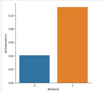
Summary

The chi-square test of independence suggests an association of alcohol dependence for those with alcoholic parents for both groups in the NESARC dataset. For those that were in the category, 21 years old and older, the chi-squared statistic was 166.27 with a p-value of < 0.001 (4.8e-38). The graph reveals that for this group, 11.3% of respondents who had alcoholic parents were alcohol dependent whereas those with no alcoholic parents were 4.1% likely. The 20 years old and younger group has a chi-squared statistic of 565.76 and a p-value of < 0.001 (4.7e-125). The category plot displays for this group, that 30.0% of those that have alcoholic parents were alcohol dependent. As opposed to those who did not have alcoholic parents, who were only 15.8% likely. Notably there is a significant increase in the likelihood of alcohol dependence for those who start drinking under the age of 21. The NESARC dataset results displayed this with an increase of 11.7% from started drinking under the age of 21 and not having an alcoholic parent(s) and an increase of 18.7% from started drinking under the age of 21 and having alcoholic parent(s) in comparison to those who started drinking from 21 and over. However, we cannot conclude that the age someone started drinking at is a key moderator, but this can help form the basis for further tests.

[thepandas]

Generating Correlation Coefficients

The topic I am looking at is the association with alcoholic parent(s) and the child becoming alcohol dependent using the NESARC dataset. The variables I have been using are predominately categorical and therefore for the purpose of this assignment I have pulled out 2 additional quantitative variables. The 3 variables I am using for my dataset are:

-       Alcohol Dependence – (Derived from Age at onset of Alcohol Dependence).

-       AgeAtHeaviestPeriod - Age at start of period of heaviest drinking

-       LargestNoOfDrinksInHeaviestPeriod - Largest Number of Drinks of any alcohol consumed on days when drank alcohol during period of heaviest drinking.

 Data Management

As per previous modules, the following code is to import the data, derive the new variables and set data types.

# import libraries

import pandas as pd

import numpy as np

import scipy

import seaborn as sns

import matplotlib.pyplot as plt

 # set display options for pandas

pd.set_option('display.max_columns', 100)

pd.set_option('display.max_rows', 100)

 # import data

df = pd.read_csv(r'nesarc_pds.csv', low_memory=False, usecols=['AGE','S2BQ2D','S2AQ8B','S2AQ21C','S2AQ19'])

 df.rename(columns={'S2BQ2D':'AgeAlcDependence','S2AQ8B':'NoOfDrinksLast12mths','S2AQ21C':'LargestNoOfDrinksInHeaviestPeriod', 'S2AQ19':'AgeAtHeaviestPeriod'}, inplace=True)

 # function for alc dependence category

def AlcDependenceCat(value):

  if (value.isnumeric()) and (value != 99):

      return 1

  else:

      return 0

 # apply function

df['AlcDependence'] = list(map(AlcDependenceCat, df['AgeAlcDependence']))

 # clean spaces to nan

df['NoOfDrinksLast12mths'].replace(r'^\s+$',np.nan, regex=True, inplace=True)

df['AGE'].replace(r'^\s+$',np.nan, regex=True, inplace=True)

df['LargestNoOfDrinksInHeaviestPeriod'].replace(r'^\s+$',np.nan, regex=True, inplace=True)

df['AgeAtHeaviestPeriod'].replace(r'^\s+$',np.nan, regex=True, inplace=True)

  df['NoOfDrinksLast12mths'] = pd.to_numeric(df['NoOfDrinksLast12mths'])

df['AGE'] = pd.to_numeric(df['AGE'])

df['LargestNoOfDrinksInHeaviestPeriod'] = pd.to_numeric(df['LargestNoOfDrinksInHeaviestPeriod'])

df['AgeAtHeaviestPeriod'] = pd.to_numeric(df['AgeAtHeaviestPeriod'])

 # only return those who are alc dependent, remove nans and 99s

df_alc_dep = df.loc[df['AlcDependence'] == 1]

data = df_alc_dep.dropna()

df2 = data.loc[(data['AgeAtHeaviestPeriod'] != 99) & (data['LargestNoOfDrinksInHeaviestPeriod'] != 99)]

 Pearson Correlation Coefficient for the Start age at Heaviest Alcohol period by Largest Number of drinks consumed within period.

print('The largest number of drinks consumered by age at the start of the heaviest drinking period (for Alcohol Dependents)')

scatter2 = sns.regplot(x='AgeAtHeaviestPeriod', y='LargestNoOfDrinksInHeaviestPeriod', fit_reg=True, data=df2)

plt.xlabel('Age at Heaviest Alc Consumption')

plt.ylabel('Largest # of Alc consumed')

plt.show()

 print('Pearson r coefficient and corresponding P-Value')

print(scipy.stats.pearsonr(df2['AgeAtHeaviestPeriod'], df2['LargestNoOfDrinksInHeaviestPeriod']))

Summary

As observed in the scatter graph produced, there is no correlation in the NESARC dataset between the Age that an alcohol dependent enters their heaviest drinking period and the largest number of alcoholic beverages consumed within their heaviest drinking period. A Pearson r correlation coefficient of -0.17 (p-value < 0.01) was produced suggesting there is no real linear relation between these 2 variables. The r-squared value results in 0.0294, this implies that we can only predict 3% of the variability of the largest number of alcohol beverages consumed when the age of heaviest alcohol consumption is known.

[thepandas]

Chi Square test of Independence

The topic I am looking at is the association with alcoholic parent(s) and the child becoming alcohol dependent using the NESARC dataset. The 2 variables that I will be using for this assignment are:

-        Alcoholic Parent(s) - (Derived from ‘Blood/Natural Father ever an alcoholic or problem drinker’ and ‘Blood/Natural Mother ever an alcoholic or problem drinker’).

-        Alcohol Dependence – (Derived from Age at onset of Alcohol Dependence).

 Data Management

As per previous modules, the following code is to import the data, derive the new variables and set data types.

# import required libraries

import pandas as pd

import numpy as np

import seaborn as sns

import matplotlib.pyplot as plt

import scipy.stats

 # set display options for pandas output

pd.set_option('display.max_rows',100)

pd.set_option('display.max_columns',100) # import data & rename columns

 # import data into dataframe

df = pd.read_csv(r'C:\Users\cgordon\Documents\training\Data Analysis - Coursera\Week 2\nesarc_pds.csv',

                usecols=['S2AQ16A','S2BQ2D','S2DQ1','S2DQ2']

                , low_memory=False)

df.rename(columns={'S2DQ1':'Father_Alcoholic', 'S2DQ2':'Mother_Alcoholic', 'S2AQ16A':'AgeStartedDrinking',

                'S2BQ2D':'AgeAlcoholDependence'}, inplace=True) True)

 def alcDependence(value):

   if (value != 99) and (value.isnumeric()):

       return 1

   elif value == 99:

       return np.nan

   else:

       return 0

  def alcParent(Father, Mother):

   if (Father == 1) | (Mother == 1):

       return 1

   else:

       return 0

 df['AlcDependence'] = list(map(alcDependence, df['AgeAlcoholDependence']))

df['AlcParents'] = list(map(alcParent, df['Father_Alcoholic'], df['Mother_Alcoholic']))

  # clean blanks

df['AgeStartedDrinking'].replace(r'^\s+$',np.nan, regex=True, inplace=True)

# correct data types for fields

df['AlcDependence'].astype('category')

df['AlcParents'].astype('category')

df['AgeStartedDrinking'] = pd.to_numeric(df['AgeStartedDrinking']) 

CHI Squared – Association between alcohol dependence and alcoholic parents.

 observed_counts = pd.crosstab(df['AlcParents'], df['AlcDependence'])

 ob_pct = observed_counts/observed_counts.sum(axis=0)

# apply chi 2 model

cs1 = scipy.stats.chi2_contingency(observed_counts)

print(cs1)

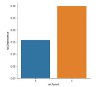
# graph alc dep % by alc parents

sns.catplot(x='AlcParents',y='AlcDependence', data=df, kind='bar', ci=None)

plt.show()

Model Summary

When conducting a chi-squared test of independence on the NESARC dataset for the association of alcohol dependence on those with alcoholic parents, the test revealed a significant dependence between the two. Those with alcoholic parents were more likely to experience alcohol dependence (22.2%) compared to those without alcoholic parents (9.0%). Chi Square statistic = 1187.70, 1 degree of freedom, p-value < 0.001.

[thepandas]

ANOVA and Post Hoc Analysis

The topic I am looking at is the association with alcoholic parent(s) and the child becoming alcohol dependent using the NESARC dataset. There are 4 variables that I am using for this research topic. I have also derived 2 new variables using 3 of the variables from the initial dataset. The 3 variables that I will be using for this assignment are:

-        Alcoholic Parent(s) - (Derived from ‘Blood/Natural Father ever an alcoholic or problem drinker’ and ‘Blood/Natural Mother ever an alcoholic or problem drinker’).

-        Alcohol Dependence – (Derived from Age at onset of Alcohol Dependence).

-        Age when started drinking.

 Data Management

As per previous modules, the following code is to import the data, derive the new variables and set data types.

# import required libraries

import pandas as pd

import numpy as np

import matplotlib.pyplot as plt

import seaborn as sns

import statsmodels.formula.api as smf

 # set output display options

pd.set_option('display.max_columns', 100)

pd.set_option('display.max_rows', 100)

 # import data & rename columns

df = pd.read_csv(r'nesarc_pds.csv',usecols=['S2AQ16A','S2BQ2D','S2DQ1','S2DQ2'] ,low_memory=False)

 df.rename(columns={'S2DQ1':'Father_Alcoholic', 'S2DQ2':'Mother_Alcoholic', 'S2AQ16A':'AgeStartedDrinking',

                  'S2BQ2D':'AgeAlcoholDependence'}, inplace=True)

 # functions for deriving new variables

def combParentAlc(father, mother):

   if (father == 1) | (mother == 1):

       return 1

   else:

       return 0

  def AlcDependence(AgeAlc):

   if (AgeAlc.isnumeric()) and (AgeAlc != 99):

       return 1

   elif AgeAlc == 99:

       return np.nan

   else:

       return 0

  df['AlcParent'] = list(map(combParentAlc, df['Father_Alcoholic'],df['Mother_Alcoholic']))

df['AlcDependence'] = list(map(AlcDependence, df['AgeAlcoholDependence']))

 # clean and set data types

df['AgeStartedDrinking'].replace(r'^\s+$', np.nan, regex=True,inplace=True)

df['AgeStartedDrinking'] = pd.to_numeric(df['AgeStartedDrinking'])

df['AlcParent'].astype('category')

df['AlcDependence'].astype('category')

 ANOVA – Association between age started drinking and alcoholic parents for those who are alcohol dependent.

 # only get respondents that have a valid drink age value and who are Alcohol dependent

df2 = df.loc[(df['AgeStartedDrinking'] != 99) & (df['AgeStartedDrinking'].notna()) & (df['AlcDependence'] == 1) ]

 # model

model = smf.ols(formula='AgeStartedDrinking ~ C(AlcParent)', data=df2)

 # fit model and produce results

results = model.fit()

print(results.summary())

print(df2.groupby('AlcParent')['AgeStartedDrinking'].mean().round(1))

Model Summary

When examining the association between Age Started Drinking and alcoholic parents for those that are alcohol dependent using the NESARC dataset, the Analysis of Variance model determined that there was a significant difference in those that have alcoholic parents and those that do not. Those who did not have an alcoholic parent had a mean age of 17.3 with a standard deviation of 3.6. Those who did have an alcoholic parent had a mean age of 16.7 with a standard deviation of 4.0. The F-statistic was 31.76 (1, 5073) with a p value of < 0.001.

ANOVA – Association between age started drinking and alcoholic parents by category for those who are alcohol dependent.

 The previous ANOVA supports my original research question, however, to apply the Post Hoc analysis I have decided to derive a new variable to apply the logic.

 The new variable breakdowns the alcoholic parent to identify the following:

1.      Where the Father is an alcoholic, but the mother is not.

2.      If both parents are alcoholic.

3.      Where the Mother is an alcoholic, but the Father is not.

4.      Where neither parent is an alcoholic.

 #new variable for alcoholic parent category

def AlcoholParentCat(father, mother):

   if (father == 1) and (mother != 1):

       return 1

   elif (father == 1) and (mother == 1):

       return 2

   elif (father != 1) and (mother == 1):

       return 3

   elif (father != 1) and (mother != 1):

       return 4

  # apply new variable, set as category, and only get those who are alcohol dependent.

df['AlcParentCategory'] = list(map(AlcoholParentCat, df['Father_Alcoholic'], df['Mother_Alcoholic']))

df['AlcParentCategory'].astype('category')

df3 = df.loc[(df['AgeStartedDrinking'] != 99) & (df['AgeStartedDrinking'].notna()) & (df['AlcDependence'] == 1) ]

 # ols model

model2 = smf.ols(formula='AgeStartedDrinking ~ C(AlcParentCategory)', data=df3)

 # fit ols model

model2 = smf.ols(formula='AgeStartedDrinking ~ C(AlcParentCategory)', data=df3)

Model Summary

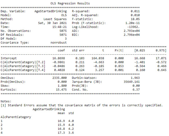
When examining the association between Age Started Drinking and the alcoholic parent’s category for those that are alcohol dependent using the NESARC dataset, the Analysis of Variance model determined that there was a significant difference. However, it is not known which groups have a significant difference. The F-statistic was 18.05 (3, 5071) and the p-value was < 0.001.

Post Hoc Analysis

# import library for Tukey’s model

import statsmodels.stats.multicomp as multi

 # apply model and print results

mc = multi.MultiComparison(df3['AgeStartedDrinking'],df3['AlcParentCategory'])

res = mc.tukeyhsd()

print(res.summary())

Post Hoc Model Summary

The Post Hoc analysis using Tukey’s Honestly significant difference test revealed that there was significant difference in the NESARC data for the age a respondent started drinking in relation to their parents for those respondents who were alcohol dependent. The test resulted in the following:

-        There was significant difference between a Father alcoholic only (mean = 16.9, std = 4.0) to both parents being alcoholics (mean=15.9, std = 4.0).

-        There was significant difference between a Father alcoholic only (mean = 16.9, std = 4.0) to neither parent being an alcoholic (mean=17.3, std = 3.6).

-        There was a significant difference between both parents being alcoholics (mean=15.9, std = 4.0) to the mother being an alcoholic (mean=16.8, std = 4.2).

-        There was a significant difference between both parents being alcoholics (mean=15.9, std = 4.0) to neither parent being an alcoholic (mean=17.3, std = 3.6).

All other comparisons were statistically similar.

[thepandas]

Graphing Univariate and Bivariate data

The topic I am looking at is the association with alcoholic parent(s) and the child becoming alcohol dependent using the NESARC dataset. There are 4 variables that I am using for this research topic. I have also derived 2 new variables using 3 of the variables from the initial dataset. The 3 variables that I will be using for this assignment are:

-        Alcoholic Parent(s) - (Derived from ‘Blood/Natural Father ever an alcoholic or problem drinker’ and ‘Blood/Natural Mother ever an alcoholic or problem drinker’).

-        Alcohol Dependence – (Derived from Age at onset of Alcohol Dependence).

-        Age when started drinking.

All Python code to generate statistics and graphs can be found in the appendix at the end.

Univariate Graph for Alcoholic Parents

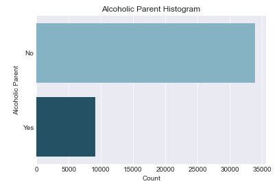
The histogram below is for the ‘Alcoholic Parent’ variable. There are only 2 outputs for this categorical variable, Yes and No. As made evident by the spread of the graph, the majority (78.7%) of respondents did not have an alcoholic parent.

Univariate Graph for Alcohol Dependence

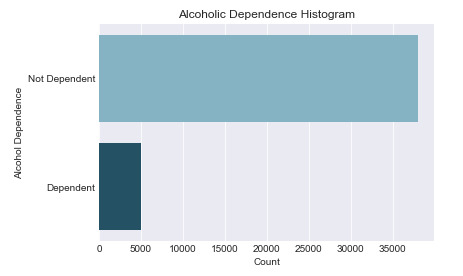
The histogram below is for the ‘Alcohol Dependence’ variable. This categorical variable only defines if a respondent is Alcohol Dependent or not. 88.4% of respondents are not dependent on alcohol which is visually represented in the graph.

Univariate Graph for Age When Started Drinking

The histogram below is for the ‘Age When Started Drinking’ variable. This variable has a unimodal distribution which peaks at an age of 18 (which is also the mode). This distribution is skewed right, where it is concentrated in early ages from 16 to 22 but tails off where there are still a few respondents who started drinking from the ages of 40 to 60. Records that return a value of 99 is where the respondents did not know the age they started drinking – excluding this for center of spread calculations, the mean average of this data is 19.7 years old and the median is 18 years old. Interestingly, even though the data is concentrated around the 18 years old mark, the data has a standard deviation of 6.1 years.    

Bivariate graph for the Alcohol dependence by Alcoholic Parents

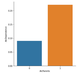
The bivariate graph below looks at the association between the categorical variable Alcoholic Parents and the categorical variable Alcohol Dependence. The graph shows that 8% of respondents who did not have an Alcoholic Parent had an Alcohol Dependence. Whereas respondents who did have an alcoholic parent were 22% likely to be Dependent on Alcohol based on the sample data.

Bivariate graph for Age started Drinking by Alcoholic Parents

The bivariate graph focuses on those respondents who are alcohol dependent, looking at the association between the Alcoholic Parents variable and the Age Started Drinking quantitative variable. The graph displays the mean for the two groups of alcoholic parents and non-alcoholic parents. The output is marginally different between the two groups with the mean age of respondents with alcoholic parents being slightly younger at 16.7 years old as opposed to non-alcoholic parent respondents at 17.3 years old.

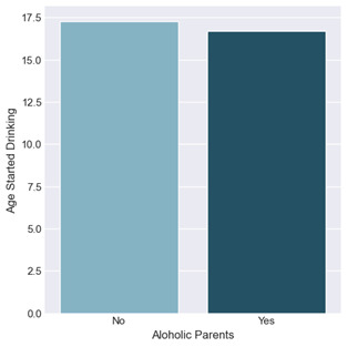
In summary, it can be seen visually that those with an alcoholic parent are more than twice as likely to be alcohol dependent based on the NESARC respondents data. However, for those that are alcohol dependent there does not appear to be a difference in the age they started drinking in relation to them having an alcoholic parent or not.  

Appendix

Python Code for data & graphs.

import pandas as pd

import numpy as np

import matplotlib.pyplot as plt

import seaborn as sns

 pd.set_option('display.max_rows',100)

 # load data

df = pd.read_csv(r'Documents\nesarc_pds.csv',usecols=['S2AQ16A','S2BQ2D','S2DQ1','S2DQ2'] ,low_memory=False)

 # rename columns

df.rename(columns={'S2DQ1':'Father_Alcoholic', 'S2DQ2':'Mother_Alcoholic', 'S2AQ16A':'AgeStartedDrinking',

                  'S2BQ2D':'AgeAlcoholDependence'}, inplace=True)

 # functions for deriving new values

def combParentAlc(Father, Mother):

  if (Father == 1) | (Mother == 1):

       return 1

  else:

       return 0

   def alcDependence(value):

  if (value.isnumeric()) and (value != '99'):

       return 1

  elif value == '99':

       return np.nan

  else:

       return 0

 # apply functions

df['alc_Parent'] = list(map(combParentAlc, df['Father_Alcoholic'], df['Mother_Alcoholic']))

 df['AlcDependence'] = list(map(alcDependence, df['AgeAlcoholDependence']))

 # replace blank values with nan

df['AgeStartedDrinking'].replace(r'^\s+$', np.nan, regex=True,inplace=True)

 #assign data types

df['alc_Parent'].astype('category')

df['AlcDependence'].astype('category')

df['AgeStartedDrinking'] = pd.to_numeric(df['AgeStartedDrinking'])

 #Generate Alcoholic Parent histogram

plt.style.use('seaborn-darkgrid')

ax = sns.countplot(y='alc_Parent', data=df, palette=['#7AB8CF','#19566E'])

plt.ylabel('Alcoholic Parent')

plt.xlabel('Count')

plt.title('Alcoholic Parent Histogram')

plt.yticks([0,1],['No','Yes'])

plt.show()

 print(df['alc_Parent'].value_counts(normalize=True).to_frame() * 100)

 #Generate alcohol dependence histogram

plt.style.use('seaborn-darkgrid')

ax = sns.countplot(y='AlcDependence', data=df, palette=['#7AB8CF','#19566E'])

plt.ylabel('Alcohol Dependence')

plt.xlabel('Count')

plt.title('Alcoholic Dependence Histogram')

plt.yticks([0,1],['Not Dependent','Dependent'])

plt.show()

 print(df['AlcDependence'].value_counts(normalize=True).to_frame())

 # generate histogram for Age Started Drinking

plt.style.use('seaborn-darkgrid')

ax = sns.distplot(df['AgeStartedDrinking'].dropna(), kde=False)

plt.xlabel('Age Started Drinking')

plt.title('Age Started Drinking Distribution')

plt.show()

 print(df['AgeStartedDrinking'].mode())

print(df.loc[df['AgeStartedDrinking'] != 99, 'AgeStartedDrinking'].median())

print(df.loc[df['AgeStartedDrinking'] != 99, 'AgeStartedDrinking'].mean())

print(df.loc[df['AgeStartedDrinking'] != 99, 'AgeStartedDrinking'].std())

 # Generate bivariate graph for Alcoholic Parents by Alcohol Dependence

plt.style.use('seaborn-darkgrid')

sns.catplot(y='AlcDependence',x='alc_Parent',data=df, kind='bar', ci=None, palette=['#7AB8CF','#19566E'])

plt.xticks([0,1], ['No','Yes'])

plt.xlabel('Alcoholic Parents')

plt.ylabel('Alcohol Dependence')

plt.show()

 # Generate bivariate graph for alc dependence responses for alc parents by age started drinking

dfAlcDep = df.loc[(df['AlcDependence'] == 1) & (df['AgeStartedDrinking'] != 99)].copy()

plt.style.use('seaborn-darkgrid')

sns.catplot(y='AgeStartedDrinking',x='alc_Parent',data=dfAlcDep, kind='bar', ci=None,palette=['#7AB8CF','#19566E'])

plt.xticks([0,1], ['No','Yes'])

plt.xlabel('Aloholic Parents')

plt.ylabel('Age Started Drinking')

plt.show()

 print(dfAlcDep.groupby('alc_Parent', as_index=False).agg({'AgeStartedDrinking':'mean'}))

[thepandas]

Making Data Management Decisions

The topic I am looking at is the association with alcoholic parent(s) and the child becoming alcohol dependent using the NESARC dataset. There are 4 variables that I am using for this research topic. I have also derived 2 new variables using 3 of the variables from the initial dataset. The 3 variables that I will be using for this assignment are:

-        Alcoholic Parent(s) - (Derived from ‘Blood/Natural Father ever an alcoholic or problem drinker’ and ‘Blood/Natural Mother ever an alcoholic or problem drinker’)

-        Alcohol Dependence – (Derived from Age at onset of Alcohol Dependence)

-        Age when started drinking

 Python Code

My Python code to produce the results is below.

 import numpy as np

import pandas as pd

 pd.set_option('display.max_rows',100)

 file = r'nesarc_pds.csv'

df = pd.read_csv(file,usecols=['S2AQ16A','S2BQ2D','S2DQ1','S2DQ2'] ,low_memory=False)

 # functions for deriving new values

def combParentAlc(Father, Mother):

   if (Father == 1) | (Mother == 1):

       return 1

   else:

       return 0

 def alcDependence(value):

   if (value.isnumeric()) and (value != '99'):

       return 1

   elif value == '99':

       return np.nan

   else:

       return 0

 df.rename(columns={'S2DQ1':'Father_Alcoholic', 'S2DQ2':'Mother_Alcoholic', 'S2AQ16A':'AgeStartedDrinking',

                  'S2BQ2D':'AgeAlcoholDependence'}, inplace=True)

 # apply functions on variables

df['alc_Parent'] = list(map(combParentAlc, df['Father_Alcoholic'], df['Mother_Alcoholic']))

 df['AlcDependence'] = list(map(alcDependence, df['AgeAlcoholDependence']))

 alc_dep = df['AlcDependence'].value_counts(dropna=False).to_frame()

alc_par = df['alc_Parent'].value_counts().to_frame()

 alc_dep['Alc_Dependence_%_of_total'] = round(alc_dep['AlcDependence']*100 / sum(alc_dep['AlcDependence']),2)

alc_par['Alc_Parent_%_of_total'] = round(alc_par['alc_Parent']*100 / sum(alc_par['alc_Parent']),2)

 alc_dep.rename(index={0.0:'No', 1.0:'Yes'}, columns={'AlcDependence':'Alc_Dependence_Count'}, inplace=True)

alc_par.rename(index={0.0:'No', 1.0:'Yes'}, columns={'alc_Parent':'Alc_Parent_Count'}, inplace=True)

 print(alc_dep)

print(alc_par)

 df['AgeStartedDrinking2'] = df['AgeStartedDrinking']

df['AgeStartedDrinking2'] = df['AgeStartedDrinking2'].replace(r'^\s+$', np.nan, regex=True)

df['AgeStartedDrinking2'] = pd.to_numeric(df['AgeStartedDrinking2'])

 bi = [10,20,30,40,50,60,70,80,90,99,100]

lab = ['10 - 20','20 - 30','30 - 40','40 - 50','50 - 60','60 - 70','70 - 80','80 - 90','90 - 99','Unknown']

df['AgeStartedDrinkingBucket'] = pd.cut(df['AgeStartedDrinking2'], bins=bi, labels=lab, right=False)

 age_drk = df['AgeStartedDrinkingBucket'].value_counts(dropna=False).sort_index().to_frame()

 age_drk['Age_Drinking_%_of_total'] = round(age_drk['AgeStartedDrinkingBucket'] *100 / sum(age_drk['AgeStartedDrinkingBucket']), 2)

 print(age_drk)

 Frequency table Output

Alcohol Dependence

Alcoholic Parent(s)

Age Started drinking

Summary

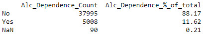
 The Alcohol Dependence variable was derived from the ‘Age at onset of Alcohol Dependence’ variable where any numeric value excluding 99 was defined as ‘Yes’, anything that was blank was ‘No’ (as per the codebook definition) and 99 which is identified as Unknown I changed to Nan (python’s equivalent of NULL). I have treated these as missing values but still want to include these records to maintain the full sample size for now. Of the total number of observations, 88.2% were not alcohol dependent and 11.6% were alcohol dependent. The remaining 0.2% (90 records) where unknown (Nan).  

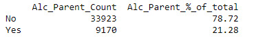
 The Alcoholic Parent(s) variable was derived from the 2 variables ‘Blood/Natural Father ever an alcoholic or problem drinker’ and ‘Blood/Natural Mother ever an alcoholic or problem drinker’. To handle missing values for these two variables, I decided to assume where it was unknown the value would be No to clean the output. From this new variable, 78.7% of observation did not have alcoholic parent(s) whereas the remaining 21.3% did.

 The ‘age started drinking’ variable was grouped into buckets, primarily using multiples of 10. The highest number of observations (46.2%) were in the age group 10-20. The second highest group was 20-30 with 26.9% of records. The remaining age groups where participants responded to the question only equated to 4.5%.  2.2% did not know the age they started drinking and 20.2% were lifetime abstainers.