ultrafahmina06things-blog

[ultrafahmina06things-blog]

Week4 - Assignment

For this assignment, Though three or more variables could be selected, in the name of clarity and simplicity and to focus on the hypothesis of the project, I opted for only 2: Life Expectancy and alcohol consumption.

Here is my code:

# importing necessary libraries

%matplotlib inline import pandas as pd import numpy as np from collections import OrderedDict from tabulate import tabulate, tabulate_formats import seaborn import matplotlib.pyplot as plt

# bug fix for display formats to avoid run time errors pd.set_option('display.float_format', lambda x:'%f'%x) # Load from CSV

data1 = pd.read_csv('D:/CourseEra/gapminder.csv', skip_blank_lines=True,                   usecols=['country',                             'alcconsumption', 'lifeexpectancy']) data1=data1.replace(r'^\s*$', np.nan, regex=True) data1 = data1.dropna(axis=0, how='any') # Variables Descriptions ALCOHOL = "2008 alcohol consumption per adult (liters, age 15+)" LIFE = "2011 life expectancy at birth (years)" for dt in ( 'alcconsumption', 'lifeexpectancy') :     data1[dt] = pd.to_numeric(data1[dt], 'errors=coerce') data2 = data1.copy()

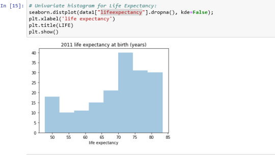
#Univariate histogram for alcohol consumption: seaborn.distplot(data1["alcconsumption"].dropna(), kde=False); plt.xlabel('alcohol consumption (liters)') plt.title(ALCOHOL) plt.show()

The univariate graph of alcohol consumption :

The Univariate Graph of Life Expectancy:

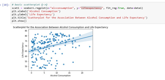
Scatterplot for the association between Alcohol Consumption and Life Expectancy:

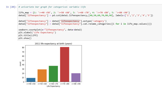
Univariate bar graph for categorical variable life expectancy:

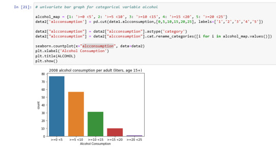
Univariate bar graph for categorical variable alcohol consumption:

Bivariate bar graph

Analyzing only the scatter graph seems do not be a correlation between the variables, but considering the bivariate bar graph, we can say that moderate alcohol consumption can contribute to life expectancy increases. Of course, this is not a scientific work and have value only for this context.

[ultrafahmina06things-blog]

Week3-Assignment

Below is the full code -

# importing necessary libraries

import pandas as pd import numpy as np from collections import OrderedDict from tabulate import tabulate, tabulate_formats

# Dictionaries

counts = OrderedDict() prcnts = OrderedDict()

# Load from CSV

data1 = pd.read_csv('D:/CourseEra/gapminder.csv', skip_blank_lines=True,                   usecols=['country','incomeperperson',                             'alcconsumption', 'lifeexpectancy'])

data1=data1.replace(r'^\s*$', np.nan, regex=True) data1 = data1.dropna(axis=0, how='any')

ALCOHOL = "2008 alcohol consumption per adult (liters, age 15+)" INCOME = "2010 Gross Domestic Product per capita in constant 2000 US$" LIFE = "2011 life expectancy at birth (years)"

for dt in ('incomeperperson', 'alcconsumption', 'lifeexpectancy') :     counts[dt] = pd.to_numeric(data1[dt], 'errors=coerce')

# absolute Frequency distributions freq_life_n = data1.lifeexpectancy.value_counts(sort=False) freq_income_n = data1.incomeperperson.value_counts(sort=False) freq_alcohol_n = data1.alcconsumption.value_counts(sort=False)

# Relative Frequency distributions freq_life_r = data1.lifeexpectancy.value_counts(sort=False, normalize=True) freq_income_r = data1.incomeperperson.value_counts(sort=False, normalize=True) freq_alcohol_r = data1.alcconsumption.value_counts(sort=False, normalize=True)

print ('********************************************************') print ('* Absolute Frequencies original variables (first 5)    *') print ('********************************************************') print ('\nlife variable ('+LIFE+'):') print ( tabulate([freq_life_n.head(5)], tablefmt="fancy_grid", headers=([i for i in freq_life_n.index])) ) print ('\nincome variable ('+INCOME+'):') print ( tabulate([freq_income_n.head(5)], tablefmt="fancy_grid", headers=([i for i in freq_income_n.index])) ) print ('\nalcohol variable ('+ALCOHOL+'):') print ( tabulate([freq_life_n.head(5)], tablefmt="fancy_grid", headers=([i for i in freq_life_n.index])) )

print ('\n********************************************************') print ('* Relative Frequencies original variables (first 5)    *') print ('********************************************************')

print ('\nlife variable ('+LIFE+'):') print ( tabulate([freq_life_r.head(5)], tablefmt="fancy_grid", headers=([i for i in freq_life_n.index])) ) print ('\nincome variable ('+INCOME+'):') print ( tabulate([freq_income_r.head(5)], tablefmt="fancy_grid", headers=([i for i in freq_income_n.index])) ) print ('\nalcohol variable ('+ALCOHOL+'):') print ( tabulate([freq_life_r.head(5)], tablefmt="fancy_grid", headers=([i for i in freq_life_n.index])) )

******************************************************** * Absolute Frequencies original variables (first 5)    * ******************************************************** life variable (2011 life expectancy at birth (years)): ╒══════════╤══════════╤══════════╤══════════╤══════════╕ │   74.402 │   73.373 │   54.675 │   81.804 │   76.126 │ ╞══════════╪══════════╪══════════╪══════════╪══════════╡ │        1 │        1 │        1 │        1 │        1 │ ╘══════════╧══════════╧══════════╧══════════╧══════════╛ income variable (2010 Gross Domestic Product per capita in constant 2000 US$): ╒════════════════════╤════════════════════╤════════════════════╤════════════════════╤════════════════════╕ │   9425.32586978275 │   15313.8593472276 │   389.763634253063 │   268.331790297681 │   11744.8341671737 │ ╞════════════════════╪════════════════════╪════════════════════╪════════════════════╪════════════════════╡ │                  1 │                  1 │                  1 │                  1 │                  1 │ ╘════════════════════╧════════════════════╧════════════════════╧════════════════════╧════════════════════╛ alcohol variable (2008 alcohol consumption per adult (liters, age 15+)): ╒══════════╤══════════╤══════════╤══════════╤══════════╕ │   74.402 │   73.373 │   54.675 │   81.804 │   76.126 │ ╞══════════╪══════════╪══════════╪══════════╪══════════╡ │        1 │        1 │        1 │        1 │        1 │ ╘══════════╧══════════╧══════════╧══════════╧══════════╛ ******************************************************** * Relative Frequencies original variables (first 5)    * ******************************************************** life variable (2011 life expectancy at birth (years)): ╒════════════╤════════════╤════════════╤════════════╤════════════╕ │     74.402 │     73.373 │     54.675 │     81.804 │     76.126 │ ╞════════════╪════════════╪════════════╪════════════╪════════════╡ │ 0.00584795 │ 0.00584795 │ 0.00584795 │ 0.00584795 │ 0.00584795 │ ╘════════════╧════════════╧════════════╧════════════╧════════════╛ income variable (2010 Gross Domestic Product per capita in constant 2000 US$): ╒════════════════════╤════════════════════╤════════════════════╤════════════════════╤════════════════════╕ │   9425.32586978275 │   15313.8593472276 │   389.763634253063 │   268.331790297681 │   11744.8341671737 │ ╞════════════════════╪════════════════════╪════════════════════╪════════════════════╪════════════════════╡ │         0.00584795 │         0.00584795 │         0.00584795 │         0.00584795 │         0.00584795 │ ╘════════════════════╧════════════════════╧════════════════════╧════════════════════╧════════════════════╛ alcohol variable (2008 alcohol consumption per adult (liters, age 15+)): ╒════════════╤════════════╤════════════╤════════════╤════════════╕ │     74.402 │     73.373 │     54.675 │     81.804 │     76.126 │ ╞════════════╪════════════╪════════════╪════════════╪════════════╡ │ 0.00584795 │ 0.00584795 │ 0.00584795 │ 0.00584795 │ 0.00584795 │ ╘════════════╧════════════╧════════════╧═════════��══╧════════════╛

# Min and Max continuous variables: min_max = OrderedDict() dict1 = OrderedDict()

dict1['min'] = data1.lifeexpectancy.min() dict1['max'] = data1.lifeexpectancy.max() min_max['lifeexpectancy'] = dict1

dict2 = OrderedDict() dict2['min'] = data1.incomeperperson.min() dict2['max'] = data1.incomeperperson.max() min_max['incomeperperson'] = dict2

dict3 = OrderedDict() dict3['min'] = data1.alcconsumption.min() dict3['max'] = data1.alcconsumption.max() min_max['alcconsumption'] = dict3

df = pd.DataFrame([min_max['incomeperperson'],min_max['lifeexpectancy'],min_max['alcconsumption']], index = ['incomeperperson','lifeexpectancy','alcconsumption']) print (tabulate(df.sort_index(axis=1, ascending=False), headers=['Var','Min','Max'])) data2 = data1.copy()

Var                  Min      Max ---------------  -------  ------- incomeperperson  103.776  952.827 lifeexpectancy    47.794   83.394 alcconsumption     0.05     9.99

# Maps incomeperperson_map = {1: '>=100  <5k', 2: '>=5k <10k', 3: '>=10k <20k', 4: '>=20K <30K', 5: '>=30K <40K', 6: '>=40K <50K' } lifeexpectancy_map = {1: '>=40 <50', 2: '>=50 <60', 3: '>=60 <70', 4: '>=70 <80', 5: '>=80 <90'} alcconsumption_map = {1: '>=0.5 <5', 2: '>=5 <10', 3: '>=10 <15', 4: '>=15 <20', 5: '>=20 <25'}

# absolute Frequency distributions

freq_life_n = data2.lifeexpectancy.value_counts(sort=False) freq_income_n = data2.incomeperperson.value_counts(sort=False) freq_alcohol_n = data2.alcconsumption.value_counts(sort=False)

freq_life_r = data2.lifeexpectancy.value_counts(sort=False, normalize=True) freq_income_r = data2.incomeperperson.value_counts(sort=False, normalize=True) freq_alcohol_r = data2.alcconsumption.value_counts(sort=False, normalize=True)

print ('************************') print ('* Absolute Frequencies *') print ('************************') print ('\nlife variable ('+LIFE+'):') print( tabulate([freq_life_n], tablefmt="fancy_grid", headers=(lifeexpectancy_map.values()))) print ('\nincome variable ('+INCOME+'):') print( tabulate([freq_income_n], tablefmt="fancy_grid", headers=(incomeperperson_map.values()))) print ('\nalcohol variable ('+ALCOHOL+'):') print( tabulate([freq_alcohol_n], tablefmt="fancy_grid", headers=(alcconsumption_map.values())))

print ('\n************************') print ('* Relative Frequencies *') print ('************************') print ('\nlife variable ('+LIFE+'):') print( tabulate([freq_life_r], tablefmt="fancy_grid", headers=(lifeexpectancy_map.values()))) print ('\nincome variable ('+INCOME+'):') print( tabulate([freq_income_r], tablefmt="fancy_grid", headers=(incomeperperson_map.values()))) print ('\nalcohol variable ('+ALCOHOL+'):') print( tabulate([freq_alcohol_r], tablefmt="fancy_grid", headers=(alcconsumption_map.values())))

************************ * Absolute Frequencies * ************************ life variable (2011 life expectancy at birth (years)): ╒════════════╤════════════╤════════════╤════════════╤════════════╕ │   >=40 <50 │   >=50 <60 │   >=60 <70 │   >=70 <80 │   >=80 <90 │ ╞════════════╪════════════╪════════════╪════════════╪════════════╡ │          8 │         28 │         35 │         80 │         20 │ ╘════════════╧════════════╧════════════╧════════════╧════════════╛ income variable (2010 Gross Domestic Product per capita in constant 2000 US$): ╒══════════════╤═════════════╤══════════════╤══════════════╤══════════════╤══════════════╕ │   >=100  <5k │   >=5k <10k │   >=10k <20k │   >=20K <30K │   >=30K <40K │   >=40K <50K │ ╞══════════════╪═════════════╪══════════════╪══════════════╪══════════════╪══════════════╡ │          110 │          24 │           15 │           12 │            9 │            0 │ ╘══════════════╧═════════════╧══════════════╧══════════════╧══════════════╧══════════════╛ alcohol variable (2008 alcohol consumption per adult (liters, age 15+)): ╒════════════╤═══════════╤════════════╤════════════╤════════════╕ │   >=0.5 <5 │   >=5 <10 │   >=10 <15 │   >=15 <20 │   >=20 <25 │ ╞════════════╪═══════════╪════════════╪════════════╪════════════╡ │         63 │        56 │         31 │         10 │          1 │ ╘════════════╧═══════════╧════════════╧════════════╧════════════╛ ************************ * Relative Frequencies * ************************ life variable (2011 life expectancy at birth (years)): ╒════════════╤════════════╤════════════╤════════════╤════════════╕ │   >=40 <50 │   >=50 <60 │   >=60 <70 │   >=70 <80 │   >=80 <90 │ ╞════════════╪════════════╪════════════╪════════════╪════════════╡ │  0.0467836 │   0.163743 │   0.204678 │   0.467836 │   0.116959 │ ╘════════════╧════════════╧════════════╧════════════╧════════════╛ income variable (2010 Gross Domestic Product per capita in constant 2000 US$): ╒══════════════╤═════════════╤══════════════╤══════════════╤══════════════╤══════════════╕ │   >=100  <5k │   >=5k <10k │   >=10k <20k │   >=20K <30K │   >=30K <40K │   >=40K <50K │ ╞══════════════╪═════════════╪══════════════╪══════════════╪══════════════╪══════════════╡ │     0.647059 │    0.141176 │    0.0882353 │    0.0705882 │    0.0529412 │            0 │ ╘══════════════╧═════════════╧══════════════╧══════════════╧══════════════╧══════════════╛ alcohol variable (2008 alcohol consumption per adult (liters, age 15+)): ╒════════════╤═══════════╤════════════╤════════════╤════════════╕ │   >=0.5 <5 │   >=5 <10 │   >=10 <15 │   >=15 <20 │   >=20 <25 │ ╞════════════╪═══════════╪════════════╪════════════╪════════════╡ │   0.391304 │  0.347826 │   0.192547 │  0.0621118 │ 0.00621118 │ ╘════════════╧═══════════╧════════════╧════════════╧════════════╛

Explanation - 

I collapsed the responses for lifeexpectancy, incomeperperson, and alcconsumption to create three new variables: life, income, and alcohol. For life, the most commonly endorsed response was 4(>=70 <80) (46.78%), meaning that most countries have a life expectancy between 70 to 80 year old. For income, the most commonly endorsed response was 1(>=100  <5k) (64.7%), meaning that more than half of the countries have income level is between 100 to 5000 dollar. For alcohol, the most commonly endorsed response was 1(>=0.5 <5) (39.68%), meaning that the alcohol consumption for most countries is .5 to 5 liters.

[ultrafahmina06things-blog]

Assignment-Week2

Bellow is my code:

# importing necessary libraries

import pandas as pd import numpy from collections import OrderedDict from tabulate import tabulate, tabulate_formats

# Dictionaries

counts = OrderedDict() prcnts = OrderedDict()

# Load from CSV

data1 = pd.read_csv('D:/CourseEra/gapminder.csv', skip_blank_lines=True,                   usecols=['country','incomeperperson',                             'alcconsumption', 'lifeexpectancy'])

# Counts missing entry

missings = [['Var', 'Missings']] for var in ('incomeperperson', 'alcconsumption', 'lifeexpectancy'):    missings.append([var, data1[var].value_counts()[' ']]) print (tabulate(missings, headers="firstrow"))

# Count each variable

for dt in ('incomeperperson', 'alcconsumption', 'lifeexpectancy') :     counts[dt] = pd.to_numeric(data1[dt], 'errors=coerce') print (counts['incomeperperson']) print (counts['alcconsumption']) print (counts['lifeexpectancy'])

# each variable as percentage

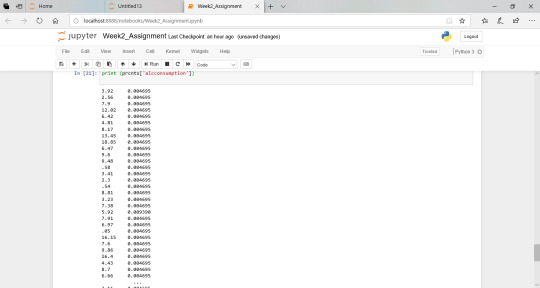
for dt in ('incomeperperson', 'alcconsumption', 'lifeexpectancy') :    prcnts[dt] = data1[dt].value_counts(sort=False, normalize=True) print (prcnts['incomeperperson']) print (prcnts['alcconsumption']) print (prcnts['lifeexpectancy'])

The output and explanation

This line shows information about dataset, where: incomeperperson alcconsumption lifeexpectancy

in the lines, 23-29 is showed the number of missing data for each variable by value_counts() function

# Counts missing entry

missings = [['Var', 'Missings']] for var in ('incomeperperson', 'alcconsumption', 'lifeexpectancy'):    missings.append([var, data1[var].value_counts()[' ']]) print (tabulate(missings, headers="firstrow"))

Var                              Missings 

 incomeperperson          23 

 alcconsumption             26

 lifeexpectancy               22

the nominal values of frequency of each observation related to the variable incomeperperson:

the nominal values of frequency of each observation related to the variable  alcconsumption:

the nominal values of frequency of each observation related to the variable lifeexpectancy:

the frequency values, of each observation related to the variable incomeperperson , expressed as a percentage

the frequency values, of each observation related to the variable alcconsumption, expressed as a percentage

the frequency values, of each observation related to the variable  lifeexpectancy , expressed as a percentage

[ultrafahmina06things-blog]

Assignment1

Data Set:

After reviewing the five provided codebooks, I have opted for the “portion of’ GapMinder. The main reason for my interest in this data set is because of the global context, especially, in regarding health data.

First Topic:

After reviewing the dataset and codebook, I want to investigate to find out the correlation between life expectancy life and alcohol consumption.

The variable I want to use here -

incomeperperson, alcconsumption and lifeexpectancy

2nd Topic:

I also want to know the possible correlation between Socioeconomic status and alcohol consumption

Research Question - Is there a direct relationship between alcohol consumption and life expectancy?

Literature Review:

I did do my research in Google Scholar with the string: “alcohol consumption life expectancy”.  My original plan was to do an in-depth investigation of the chosen topics. Due to the short time and the fact that most articles are accessible only through pay assign, I opted by to select some papers and to analyze their abstracts and the open sections (frequently, “results’’ and “conclusions”). Two of these papers are summarized below.

Drinking Pattern and Mortality:: The Italian Risk Factor and Life Expectancy Pooling Project [1]

The purpose of this article is exactly to analyze the relationship between a particular aspect of drink pattern and risk of all-cause and specific-cause mortality The results presented in this paper indicate that drinking patterns may have important health implications, impacting directly on the life expectancy.

Alcohol-related mortality by age and sex and its impact on life expectancy. Estimates based on the Finnish death register [2]

This study was made in Finland and based on the “Finnish Death Register” that includes information on both the underlying and contributory causes of death and it yields an individual-level estimate of the contribution of alcohol to mortality. The data for 1987-1993 is used to examine alcohol-related mortality by cause of death. According to the results, 6% of all deaths were alcohol-related. These deaths were responsible for a 2-year loss in life expectancy at age 15 years among men and 0.4 years among women.

Hypothesizes -

Primary hypothesis:

The level of alcohol consumption of a country might be directly related to expectancy life.

Secondary hypothesis:

Socioeconomic status and income levels have a direct correlation with the level of alcohol consumption of a country.

[ultrafahmina06things-blog]

dfd