uspscourse

[uspscourse]

Capstone Project - F3

Results

Descriptive Statistics

Table 1 shows descriptive statistics for export goods and services (highlighted in green) among countries and the quantitative predictors. The average export goods and services was 43.97% (Std Dev=28.89), with a minimum export of 5.52 % and a maximum of 225.56

Bivariate Analyses

Scatter and box plots for the association between the export of goods and services response variable and quantitative predictors (Figure 1 and Figure 2) revealed that export of goods and services were not strongly related with any of the predictor’s variables. The one area showed correlation is AGRICULTURE_VALUE (Coef = -0.1261, p < 0.0369) as showed with the ANOVA results indicated.

FOREIGN_INVESTMENT (Coef = 0.0520, p < 0.2804)

INDUSTRY_VALUE (Coef = -0.0220, p < 0.5609)

MANUFACTURE_VALUE (Coef = 0.0289, p < 0.6633)

GDP_GROWTH (Coef = 0.0126, p < 0.9243)

Figure 1: Association between export goods and service and quantitative predictors

Figure 2: Association between export goods and service and quantitative predictors

Lasso and R2 Regression Analysis

I used the Coefficient of Determination also popularly known as R square value is a regression error metric to evaluate the accuracy and efficiency of a model on the data. R square values describe the performance of the model. It describes the variation in the response or target variable which is predicted by the independent variables of the data model. R square value helps determine how well the model is blend and how well the output value is explained by the determining(independent) variables of the dataset. The value of R square ranges between [0,1]. Higher is the R square value, better is the model and the results. Base on the output of the R2 score plot, the 1st training (0.51994647) and test (0.2165552) R2 score model was not close to the normal (0.95717998). (Figure 3 and Table 2).

Figure 3: R2 Score of each model

Standardized training data (MSE = 3.7089) and test data (MSE = 3.7982) were essentially the same which suggested that predictive accuracy did not decline when the lasso regression algorithm developed on the training data set was applied to predict export of goods and services in the test data set.

[uspscourse]

Capstone Project - F2

Methods

 Sample

 The data collected by the World Bank dataset for year 2012 which last modified on 03/11/2016 was used to conduct this sample. It contains 248 observations (Countries) and 163 variables which 6 were being used for analysis.

 Measures

 The collected manufactory, industry and agriculture value data were used to measure the relation between them and export goods and services volume (high, lower, or no effect). The direct foreign investment data was used to measure higher direct investment from outside a country did resulting in higher export of goods and services. Finally, by measuring the food productivity and electricity accessibility measured a country’s ability to produce good and services for export.

 Analyses

 The distributions for the predictors and the export goods and services response variable were evaluated by calculating the mean, standard deviation, minimum and maximum values for quantitative variables. Scatter plots and box plots were also examined, and Pearson correlation and Analysis of variance (ANOVA) were used to test bivariate associations between individual predictors and the export goods and services response variable. Lasso regression with the least angle regression selection algorithm was used to identify the subset of variables that shows strong relation or not to export goods and services. The lasso regression model was estimated on a training data set consisting of a random sample of 70% of the data (N=174), and a test data set included the other 30% of the batches (N=74). All predictor variables were standardized to have a mean=0 and standard deviation=1 prior to conducting the lasso regression analysis. Cross validation was performed using k-fold cross validation specifying 10 folds. The change in the cross validation mean squared error rate at each step was used to identify the best subset of predictor variables. Predictive accuracy was assessed by determining the mean squared error rate of the training data prediction algorithm when applied to observations in the test data set.

[uspscourse]

Capstone Project - F1

Report Title

The Association Between Exports of Goods / Services and Foreign Direct Investment

Introduction to the Research Question

The purpose of this study was to identify the best predictors of higher export of good and services resulting from following relation to a country’s manufactory, industry, agriculture value, electricity accessibility, food production and foreign direct investment into the country. I was interested to find out if any of these factors play any part in showing of a country’s higher, lower or not affecting export of good and services.

[uspscourse]

Machine Learning C1W4

Dataset: Gapminder.csv

A k-means cluster analysis was conducted to identify underlying subgroups of adolescents based on their similarity of responses on 10 variables that represent characteristics that could have an impact on employ rate. 

Data were randomly split into a training set that included 70% of the observations and a test set that included 30% of the observations.

Elbow curve of r-square values for the nine cluster solutions

The elbow curve was inconclusive, suggesting that the 2, 3, 6 and 8-cluster solutions might be interpreted.

Canonical discriminant analyses was used to reduce the 10 clustering variable down a few variables that accounted for most of the variance in the clustering variables. A scatterplot of the first two canonical variables by cluster shown below indicated that the observations of three clusters. They are densely packed with relatively low within cluster variance, and did not overlap very much with the other clusters. The results of this plot suggest that the best cluster solution may have fewer than 3 clusters, so it will be especially important to also evaluate the cluster solutions with fewer than 3 clusters.  

Plot of the first two canonical variables for the clustering variables by cluster

In order to externally validate the clusters, an Analysis of Variance (ANOVA) was conducting to test for significant differences between the clusters on employrate (coef=62, p=0) and clustering variable means by cluster.

Means for employrate by cluster

Standard deviations for employrate by cluster

Multiple Comparison of Means

[uspscourse]

Machine Learning C1W3

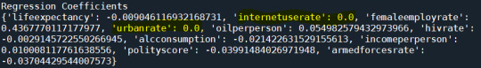
Dataset: Gapminder.csv Target variable: employrate (bin into 3 level categorical) Predictor variables: 'lifeexpectancy', 'internetuserate', 'femaleemployrate', 'urbanrate', 'oilperperson',  'hivrate', 'alcconsumption', 'incomeperperson', 'polityscore', 'armedforcesrate'

*******************************************************************************************

Data: Target (y) and predictors (X1)

Here's a simple lasso regression analysis on the gapminder dataset. It is to identify a subset of variables from a pool of 10 quantitative predictor variables that use to measure the employ rate. All predictor variables were standardized to have a mean of zero and a standard deviation of one.

Data were randomly split into a training set that included 70% of the observations and a test set that included 30% of the observations.

As the regression coefficients show below, 'internetuserate': 0.0 and 'urbanrate': 0.0 did not included in the final model due to they have a 0 coef. 'femaleemployrate' shows strongly assoicated with employrate.

The least angle regression algorithm with k=10 fold cross validation was used to estimate the lasso regression model in the training set, and the model was validated using the test set.

The change in the cross validation average (mean) squared error at each step was used to identify the best subset of predictor variables.

Regression Coefficients Progression for Lasso Paths

Change in the validation mean square error at each step

[uspscourse]

Machine Learning C1W2

Dataset: Gapminder Target Variable: employrate_bin (employrate bin into 3 categorical from quantantive) Explanatory Variables:

Matrix, Accuracy, and Classification Report

Relative Importance

Random Forest

Summary Random forest analysis was performed to evaluate the importance of a series of explanatory variables in predicting a binary, categorical response variable (employrate_bin) against the explanatory variables show above.

The explanatory variable with the highest consistent relative importance scores was female employ rate. The accuracy of the random forest was over 85%, with the subsequent growing of multiple trees rather than a single tree, adding little to the overall accuracy of the model.

[uspscourse]

Machine Learning C1W1

Program Code

Decision Tree Visualization

Summarize This decision tree is base on the train data (50% sample) from Gapminder. I had focus on three variables, two explanatory (internetuserate and lifeexpectancy) and a target variable (employrate) which I bin into 3 categories (<=50, <=75 and > 75).

As the tree shows starting from the root X[1] node,  decision will move to left leaf node if the weight is less or equal to 66.5 and move to the right leaf node if greater. The process continues until it finishes.

[uspscourse]

Data Analyst Gapminder_C3W4

Analyst: Life expectancy , internet use rate and employment rate

Bin quantitative variable employrate into 2 categories   0 for 50 and less   1 for greater than 50

One explanatory variable logistic regression p-value

One explanatory variable  odds ratio and with 95% confidence intervals

Two explanatory variables logistic regression p-value 

Two explanatory variable odds ratio and with 95% confidence intervals

Summarize: Base on the odds ratios and confidence intervals for the odds ratios (95% is between standardized residual 1.01 and 1.03) and p-value of 0, life expectancy (explanatory variable) is correlated with employ rate. Adding the explanatory variable internet use rate into the analysis, life expectancy basically stay correlated. Internet use rate, however is not as highly correlated with 95% confidence intervals for the odds ratios between 0.98 and 1.01. The p-value is 0.48. It is not acting as a confounding variable because it did not affect the correlation between the original dependent / independent variables.

[uspscourse]

Data Analyst Gapminder_C3W3

Analyst: Life expectancy , internet use rate and employment rate

q-q plot

2nd order scatter plot

Standardized residuals for all observations

Regression diagnostic plots

Leverage plot 

Ols regression results

Summarize: Base on the linear regression models and results, qq plot for normality,  influence leverage plot and plot of residuals (95% is between standardized residual -2 and 2), life expectancy is correlated with internet use rate. The regression coefficients is 2.17 and p-values is 0.000.It is interesting that employrate not correlated (p value equal 0.702 and coefficients is 0.0440) when adding it as a variable.

[uspscourse]

Data Analyst Gapminder_C3W2

Analyst: Life expectancy and employment rate

Center quantitative explanatory variable: lifeexpectancy

Linear regression model

Summarize: Base on the linear regression model with explanatory variable centered, it shows life expectancy is correlated with employment rate. The regression coefficients is 0.4979 and p-values is 0.000. 

[uspscourse]

Data Analyst Gapminder_C3W1

Sample

The Gapminder sample contains 197 countries (and territories) recognized by the UN which include 193 member states, 2 observing states, Hong Kong and Taiwan. The sample break down to four regions: The Americas, Europe, Asia, and Africa. It focus on income, health, environment, employment, technology, and life gaps. The 197 countries being use as the index of the dataset.

Procedure

The Gapminder sample was collected by asking thousands of fact questions to the public in many countries to see what people think the world looks like based on the news stories they see. The foundation also check the data from the United Nation and other reliable sources such as World Health Organization, IHME and GHDE to identify the most common misconceptions where peoples' ideas differ most from reality.

Measures

I focus my analyst on measures of employrate (This is for 2007 total employees age 15+ (% of population) Percentage of total population, age above 15, that has been employed during the given year) and internetuserate (This variable for 2010 Internet users (per 100 people) Internet users are people with access to the worldwide network) leading to higher lifeexpectancy (This variable for 2011 life expectancy at birth (years) The average number of years a newborn child would live if current mortality patterns were to stay the same) or not. My goal is to analyst the given data to find out if life expectancy is related to employ and internet use rate. Higher life expectancy equal to wealthier countries?

[uspscourse]

Data Analyst Gapminder_C3_W1 Sample The Gapminder sample contains 197 countries (and territories) recognised by the UN which include 193 member states, 2 observing states, Hong Kong and Taiwan. The sample break down to four regions: The Americas, Europe, Asia, and Aftrica. It focus on income, health, environment, employment, technology, and life gaps. The 197 countries being use as the index of the dataset. Procedure The Gapminder sample was collected by asking thousands of fact questions to the public in many countries to see what people think the world looks like based on the news stories they see. The foundation also check the data from the United Nation and other reliable sources such as World Health Organization, IHME and GHDE to identify the most common misconceptions where peoples' ideas differ most from reality. Measures I focus my analyst on measures of employrate (This is for 2007 total employees age 15+ (% of population) Percentage of total population, age above 15, that has been employed during the given year) and internetuserate (This variable for 2010 Internet users (per 100 people) Internet users are people with access to the worldwide network) leading to higher lifeexpectancy (This variable for 2011 life expectancy at birth (years) The average number of years a newborn child would live if current mortality patterns were to stay the same) or not. My goal is to analyst the given data to find out if life expectancy is related to employ and internet use rate. Higher life expectancy equal to wealther countries?

[uspscourse]

Data Analyst - Gapminder 2v4

1) Program: Gapminder2v4.py

import pandas import numpy import scipy import statsmodels.formula.api as sf_api import statsmodels.stats.multicomp as ssmc import seaborn import matplotlib.pyplot as plt

""" any additional libraries would be imported here """

""" function to group internet use rate base useage: le 25, 50, 75 and gt 75% """ def net_grp(row):    if row['internetuserate'] <= 25:        return 1    elif row['internetuserate'] <= 50:        return 2    elif row['internetuserate'] <= 75:        return 3    elif row['internetuserate'] > 75:        return 4        else:        print('Invaild data')  

""" Set PANDAS to show all columns in DataFrame """ pandas.set_option('display.max_columns', None)

"""Set PANDAS to show all rows in DataFrame """ pandas.set_option('display.max_rows', None)

""" bug fix for display formats to avoid run time errors """ pandas.set_option('display.float_format', lambda x:'%f'%x)

""" read in csv file """ data = pandas.read_csv('gapminder.csv', low_memory=False) data = data.replace(r'^\s*$', numpy.NaN, regex=True)

""" checking the format of your variables """ data['country'].dtype

""" setting variables you will be working with to numeric """ data['employrate'] = pandas.to_numeric(data['employrate'], errors='coerce') data['internetuserate'] = pandas.to_numeric(data['internetuserate'], errors='coerce') data['lifeexpectancy'] = pandas.to_numeric(data['lifeexpectancy'], errors='coerce')

""" make a copy of subset data 1 """ sub1=data.copy()

""" replace NaN to 0 and recoding to interger """ sub1['employrate'].fillna(0, inplace=True) sub1['internetuserate'].fillna(0, inplace=True) sub1['lifeexpectancy'].fillna(0, inplace=True) sub1['employrate']=sub1['employrate'].astype(int) sub1['internetuserate']=sub1['internetuserate'].astype(int) sub1['lifeexpectancy']=sub1['lifeexpectancy'].astype(int)

""" group data """ employ_gp=sub1.groupby('employrate').size() print("group employ rate among countries") print(employ_gp) net_gp=sub1.groupby('internetuserate').size()   print("group internet use rate among countries") print(net_gp) life_gp=sub1.groupby('lifeexpectancy').size() print("group life expectancy among countries") print(life_gp)

""" divde internet use rate into: 1 for <=25, 2 for <=50, 3 for <= 75, and 4 > 75% """ data_clean=sub1.dropna() line = '***************************************************************' data_clean['net_grp'] = data_clean.apply (lambda row: net_grp (row),axis=1)

""" group internetuserate into: 1 for <=25, 2 for <=50, 3 for <= 75, and 4 > 75% """ net_le25 = data_clean[(data_clean['net_grp'] == 1)] net_le50 = data_clean[(data_clean['net_grp'] == 2)] net_le75 = data_clean[(data_clean['net_grp'] == 3)] net_gt75 = data_clean[(data_clean['net_grp'] == 4)]

chk = data_clean['net_grp'].value_counts(sort=False, dropna=False) print('group internet use rate count: 1 for <=25, 2 for <=50, 3 for <= 75, and 4 > 75%') print(chk)

""" display association between lifeexpectancy and employrate base on grouped internetuserate """ stats_le25 = scipy.stats.pearsonr(net_le25['lifeexpectancy'], net_le25['employrate']) stats_le50 = scipy.stats.pearsonr(net_le50['lifeexpectancy'], net_le50['employrate']) stats_le75 = scipy.stats.pearsonr(net_le75['lifeexpectancy'], net_le75['employrate']) stats_gt75 = scipy.stats.pearsonr(net_gt75['lifeexpectancy'], net_gt75['employrate']) print ('association between lifeexpectancy and employrate for le 25% internet use rate countries') print (stats_le25) print (line) print ('association between lifeexpectancy and employrate for le 50% internet use rate countries') print (stats_le50) print (line) print ('association between lifeexpectancy and employrate for le 75% internet use rate countries') print (stats_le75) print (line) print ('association between lifeexpectancy and employrate for gt 75% internet use rate countries') print (stats_gt75)

""" scatter plot for internet use rate: 1 for <=25, 2 for <=50, 3 for <= 75, and 4 > 75% """ """ internet use rate <= 25% """ scat_le25 = seaborn.regplot(x="lifeexpectancy", y="employrate", data=net_le25) plt.xlabel('Life Expectancy') plt.ylabel('Employ Rate') plt.title('Scatterplot for the Association Between Life Expectancy and Employ Rate for le 25% Internet Use Rate') print(scat_le25) """ internet use rate <= 50% """ scat_le50 = seaborn.regplot(x="lifeexpectancy", y="employrate", data=net_le50) plt.xlabel('Life Expectancy') plt.ylabel('Employ Rate') plt.title('Scatterplot for the Association Between Life Expectancy and Employ Rate for le 50% Internet Use Rate') print(scat_le50) """ internet use rate <= 75% """ scat_le75 = seaborn.regplot(x="lifeexpectancy", y="employrate", data=net_le75) plt.xlabel('Life Expectancy') plt.ylabel('Employ Rate') plt.title('Scatterplot for the Association Between Life Expectancy and Employ Rate for le 75% Internet Use Rate') print(scat_le75) """ internet use rate >= 75% """ scat_gt75 = seaborn.regplot(x="lifeexpectancy", y="employrate", data=net_gt75) plt.xlabel('Life Expectancy') plt.ylabel('Employ Rate') plt.title('Scatterplot for the Association Between Life Expectancy and Employ Rate for gt 75% Internet Use Rate') print(scat_gt75)

2) Output: Correlation coefficent with moderator

group employ rate among countries employrate 0     35 32     1 34     1 37     1 38     1 39     1 40     1 41     3 42     5 43     1 44     4 45     1 46     6 47     5 48     4 49     2 50     4 51     6 52     3 53     6 54     4 55     7 56     9 57     7 58    11 59    10 60     5 61     8 62     3 63     8 64     5 65     7 66     6 67     1 68     4 70     2 71     5 72     2 73     3 74     1 75     2 76     1 77     1 78     3 79     1 80     1 81     2 83     3 dtype: int64 group internet use rate among countries internetuserate 0     26 1      5 2      9 3      5 4      2 5      5 6      5 7      5 8      2 9      6 10     2 11     5 12     7 13     3 14     2 15     3 16     1 18     1 19     3 20     3 21     1 24     1 25     2 26     3 27     1 28     4 29     2 31     3 32     1 33     2 34     2 35     1 36     5 38     2 39     2 40     5 41     2 42     3 43     2 44     4 45     2 46     1 47     2 48     2 49     2 51     3 52     1 53     2 54     1 56     2 60     1 61     1 62     2 63     2 65     4 66     1 68     1 69     2 70     1 71     3 72     1 73     1 74     2 75     2 76     1 77     3 79     1 80     2 81     3 82     3 83     1 84     2 86     1 88     1 90     3 93     1 95     1 dtype: int64 group life expectancy among countries lifeexpectancy 0     22 47     1 48     6 49     2 50     2 51     7 52     1 53     1 54     4 55     3 56     2 57     4 58     3 59     2 61     3 62     5 63     1 64     3 65     4 66     2 67     6 68     9 69     5 70     4 71     2 72    11 73    17 74    16 75    11 76    12 77     3 78     4 79    12 80    10 81    10 82     2 83     1 dtype: int64 group internet use rate count: 1 for <=25, 2 for <=50, 3 for <= 75, and 4 > 75% 1    10 2    18 3    13 4    15 Name: net_grp, dtype: int64 association between lifeexpectancy and employrate for le 25% internet use rate countries (0.5521857689138426, 0.09790772865774817) *************************************************************** association between lifeexpectancy and employrate for le 50% internet use rate countries (-0.21559461918908612, 0.3902333825345498) *************************************************************** association between lifeexpectancy and employrate for le 75% internet use rate countries (0.25202000730551677, 0.4061731215704616) *************************************************************** association between lifeexpectancy and employrate for gt 75% internet use rate countries (-0.010037263252458522, 0.9716793509118232)

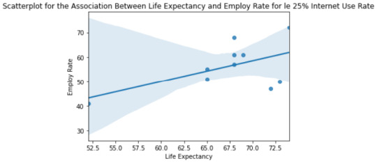
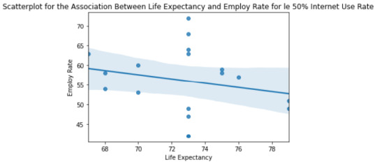
3) Testing the variables employrate and lifeexpectancy of countries on grouping the internetuserate into 4 groups: le 25, 50, 75 and gt 75%. Association produced between lifeexpectancy and employrate base on these 4 groups of internet usage (see output on item two for more details)

[uspscourse]

Data Analyst - Gapminder 2v3

1) Program: Gapminder2v3.py

import pandas import numpy import scipy import statsmodels.formula.api as sf_api import seaborn import matplotlib.pyplot as plt

""" any additional libraries would be imported here """

""" Set PANDAS to show all columns in DataFrame """ pandas.set_option('display.max_columns', None)

"""Set PANDAS to show all rows in DataFrame """ pandas.set_option('display.max_rows', None)

""" bug fix for display formats to avoid run time errors """ pandas.set_option('display.float_format', lambda x:'%f'%x)

""" read in csv file """ data = pandas.read_csv('gapminder.csv', low_memory=False) data = data.replace(r'^\s*$', numpy.NaN, regex=True)

""" checking the format of your variables """ data['country'].dtype

""" setting variables you will be working with to numeric """ data['employrate'] = pandas.to_numeric(data['employrate'], errors='coerce') data['internetuserate'] = pandas.to_numeric(data['internetuserate'], errors='coerce') data['lifeexpectancy'] = pandas.to_numeric(data['lifeexpectancy'], errors='coerce')

""" replace NaN to 0 and recoding to interger """ data['employrate'].fillna(0, inplace=True) data['internetuserate'].fillna(0, inplace=True) data['lifeexpectancy'].fillna(0, inplace=True) data['employrate']=data['employrate'].astype(int) data['internetuserate']=data['internetuserate'].astype(int) data['lifeexpectancy']=data['lifeexpectancy'].astype(int)

""" group data """ employ_gp=data.groupby('employrate').size() print("group employ rate among countries") print(employ_gp) net_gp=data.groupby('internetuserate').size()   print("group internet use rate among countries") print(net_gp) life_gp=data.groupby('lifeexpectancy').size() print("group life expectancy among countries") print(life_gp)

""" use ols function for F-statistic and associated p-value """ model_a = sf_api.ols(formula='employrate ~ C(internetuserate)', data=data).fit() print(model_a.summary())

""" Scatter Plot For Association Between Employ and Internet Use Rate """ seaborn.regplot(x='employrate', y='internetuserate', fit_reg=True, data=data) plt.xlabel('Employ Rate') plt.ylabel('Internet Use Rate') plt.title('Scatter Plot For Association Between Employ and Internet Use Rate') plt.show()

""" Scatter Plot For Association Between Life Expectancy and Internet Use Rate """ seaborn.regplot(x='lifeexpectancy', y='internetuserate', fit_reg=True, data=data) plt.xlabel('Life Expectancy') plt.ylabel('Internet Use Rate') plt.title('Scatter Plot For Association Between Life Expectancy and Internet Use Rate') plt.show()

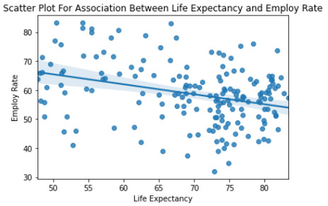
""" Scatter Plot For Association Between Life Expectancy and Employ Rate """ seaborn.regplot(x='lifeexpectancy', y='employrate', fit_reg=True, data=data) plt.xlabel('Life Expectancy') plt.ylabel('Employ Rate') plt.title('Scatter Plot For Association Between Life Expectancy and Employ Rate') plt.show()

""" fnd association between two variables """ data_clean=data.dropna()

print('Association between employ and internet use rate') print(scipy.stats.pearsonr(data_clean['employrate'], data_clean['internetuserate']))

print('Association between employ rate and life expectancy') print(scipy.stats.pearsonr(data_clean['employrate'], data_clean['lifeexpectancy']))

print('Association between employ internet use rate and life expectancy') print(scipy.stats.pearsonr(data_clean['internetuserate'], data_clean['lifeexpectancy']))

2) Output: Correlation coefficient

                           OLS Regression Results                             ============================================================================== Dep. Variable:             employrate   R-squared:                       0.387 Model:                            OLS   Adj. R-squared:                  0.045 Method:                 Least Squares   F-statistic:                     1.130 Date:                Sat, 27 Feb 2021   Prob (F-statistic):              0.266 Time:                        09:29:21   Log-Likelihood:                -923.45 No. Observations:                 213   AIC:                             2001. Df Residuals:                     136   BIC:                             2260. Df Model:                          76                                        

============================================================================== Omnibus:                        5.199   Durbin-Watson:                   2.181 Prob(Omnibus):                  0.074   Jarque-Bera (JB):                4.821 Skew:                          -0.332   Prob(JB):                       0.0898 Kurtosis:                       3.318   Cond. No.                         27.7 ==============================================================================

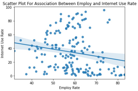
Notes: [1] Standard Errors assume that the covariance matrix of the errors is correctly specified. Association between employ and internet use rate (0.19505368645603788, 0.14969632618745277) Association between employ rate and life expectancy (0.2131830607630371, 0.11467385943527217) Association between employ internet use rate and life expectancy (0.7732949167937048, 2.8500749301451226e-12)

3) Testing the variables employrate, internetuserate and life expectancy for corretlation coefficient of all countries via scatter plots and stats (see output on item two for more details).

[uspscourse]

Data Analyst 2v2

1) Program: Gapminder2v2.py

import pandas import numpy import scipy.stats import statsmodels.formula.api as sf_api import seaborn import matplotlib.pyplot as plt

""" any additional libraries would be imported here """

""" Set PANDAS to show all columns in DataFrame """ pandas.set_option('display.max_columns', None)

"""Set PANDAS to show all rows in DataFrame """ pandas.set_option('display.max_rows', None)

""" bug fix for display formats to avoid run time errors """ pandas.set_option('display.float_format', lambda x:'%f'%x)

""" read in csv file """ data = pandas.read_csv('gapminder.csv', low_memory=False) data = data.replace(r'^\s*$', numpy.NaN, regex=True)

""" checking the format of your variables """ data['country'].dtype

""" setting variables you will be working with to numeric """ data['employrate'] = pandas.to_numeric(data['employrate'], errors='coerce') data['internetuserate'] = pandas.to_numeric(data['internetuserate'], errors='coerce') data['lifeexpectancy'] = pandas.to_numeric(data['lifeexpectancy'], errors='coerce')

"""  subset of employrate less than 76 percent, internetuserate between  25 - 75 percent and lifeexpectancy between 50 - 75 years   """ sub1=data[(data['employrate'] <= 75) & (data['lifeexpectancy'] > 50) \     & (data['lifeexpectancy'] <= 75) & (data['internetuserate'] > 50) \     & (data['internetuserate'] <= 75)]

""" make a copy of subset data 1 """ sub2=sub1.copy()

""" recoding - replace NaN to 0 and recoding to interger """ sub2['employrate'].fillna(0, inplace=True) sub2['internetuserate'].fillna(0, inplace=True) sub2['lifeexpectancy'].fillna(0, inplace=True) sub2['employrate']=sub1['employrate'].astype(int) sub2['internetuserate']=sub1['internetuserate'].astype(int) sub2['lifeexpectancy']=sub1['lifeexpectancy'].astype(int)

""" recode quantitative variable to categorical to practice chi-square  """ sub2['employrate'].astype('category') sub2['internetuserate'].astype('category')

""" use ols function for F-statistic and associated p-value """ model_a = sf_api.ols(formula='employrate ~ C(internetuserate)', data=sub2).fit() print(model_a.summary())

sub3=sub2[['employrate', 'internetuserate']].dropna().astype(int)

""" contingency table of observed counts """ print("contingency table of observed counts") oc=pandas.crosstab(sub3['employrate'], sub3['internetuserate']) print(oc)

""" column percentages """ colpct=oc/oc.sum(axis=0) print("column percentages of contingency table") print(colpct)

""" chi-square test of independence """ print("chi-square, p value, expected counts") cs=scipy.stats.chi2_contingency(oc) print(cs)

2) Output: Chi-Square Test of Independence

                           OLS Regression Results                             ============================================================================== Dep. Variable:             employrate   R-squared:                       1.000 Model:                            OLS   Adj. R-squared:                    nan Method:                 Least Squares   F-statistic:                       nan Date:                Fri, 26 Feb 2021   Prob (F-statistic):                nan Time:                        18:03:05   Log-Likelihood:                 219.29 No. Observations:                   7   AIC:                            -424.6 Df Residuals:                       0   BIC:                            -425.0 Df Model:                           6                                         Covariance Type:            nonrobust                                         ============================================================================================                               coef    std err          t      P>|t|      [0.025      0.975] -------------------------------------------------------------------------------------------- Intercept                   34.0000        inf          0        nan         nan         nan C(internetuserate)[T.56]    26.0000        inf          0        nan         nan         nan C(internetuserate)[T.61]    16.0000        inf          0        nan         nan         nan C(internetuserate)[T.62]    19.0000        inf          0        nan         nan         nan C(internetuserate)[T.65]    13.0000        inf          0        nan         nan         nan C(internetuserate)[T.71]    22.0000        inf          0        nan         nan         nan C(internetuserate)[T.74]    22.0000        inf          0        nan         nan         nan ============================================================================== Omnibus:                          nan   Durbin-Watson:                   1.400 Prob(Omnibus):                    nan   Jarque-Bera (JB):                0.749 Skew:                          -0.272   Prob(JB):                        0.688 Kurtosis:                       1.493   Cond. No.                         7.87 ==============================================================================

Notes: [1] Standard Errors assume that the covariance matrix of the errors is correctly specified. contingency table of observed counts internetuserate  51  56  61  62  65  71  74 employrate                                 34                1   0   0   0   0   0   0 47                0   0   0   0   1   0   0 50                0   0   1   0   0   0   0 53                0   0   0   1   0   0   0 56                0   0   0   0   0   1   1 60                0   1   0   0   0   0   0 column percentages of contingency table internetuserate       51       56       61       62       65       71       74 employrate                                                                     34              1.000000 0.000000 0.000000 0.000000 0.000000 0.000000 0.000000 47              0.000000 0.000000 0.000000 0.000000 1.000000 0.000000 0.000000 50              0.000000 0.000000 1.000000 0.000000 0.000000 0.000000 0.000000 53              0.000000 0.000000 0.000000 1.000000 0.000000 0.000000 0.000000 56              0.000000 0.000000 0.000000 0.000000 0.000000 1.000000 1.000000 60              0.000000 1.000000 0.000000 0.000000 0.000000 0.000000 0.000000 chi-square, p value, expected counts (35.000000000000014, 0.24264043734973734, 30, array([       [0.14285714, 0.14285714, 0.14285714, 0.14285714, 0.14285714,        0.14285714, 0.14285714],       [0.14285714, 0.14285714, 0.14285714, 0.14285714, 0.14285714,        0.14285714, 0.14285714],       [0.14285714, 0.14285714, 0.14285714, 0.14285714, 0.14285714,        0.14285714, 0.14285714],       [0.14285714, 0.14285714, 0.14285714, 0.14285714, 0.14285714,        0.14285714, 0.14285714],       [0.28571429, 0.28571429, 0.28571429, 0.28571429, 0.28571429,        0.28571429, 0.28571429],       [0.14285714, 0.14285714, 0.14285714, 0.14285714, 0.14285714,        0.14285714, 0.14285714]]))

3) Testing the variables employrate and internetuserate of countries with under 75% employ rate and between 50 - 75% internet use rate which I convert from quantitative to categorical and float to interger for this exercise. I produced the contingency table (in percentage form as well) of observed counts and the chi-square, p value and expected counts for this effort (see output on item two for more details)

[uspscourse]

Data Analyst 2v1

1) Program: Gapminder2v1.py

import pandas import numpy import statsmodels.formula.api as sf_api

""" any additional libraries would be imported here """

""" Set PANDAS to show all columns in DataFrame """ pandas.set_option('display.max_columns', None)

"""Set PANDAS to show all rows in DataFrame """ pandas.set_option('display.max_rows', None)

""" bug fix for display formats to avoid run time errors """ pandas.set_option('display.float_format', lambda x:'%f'%x)

""" read in csv file """ data = pandas.read_csv('gapminder.csv', low_memory=False) data = data.replace(r'^\s*$', numpy.NaN, regex=True)

""" checking the format of your variables """ data['country'].dtype

""" setting variables you will be working with to numeric """ data['employrate'] = pandas.to_numeric(data['employrate'], errors='coerce') data['internetuserate'] = pandas.to_numeric(data['internetuserate'], errors='coerce') data['lifeexpectancy'] = pandas.to_numeric(data['lifeexpectancy'], errors='coerce')

"""  subset of employrate less than 76 percent, internetuserate between  25 - 75 percent and lifeexpectancy between 50 - 75 years   """ sub1=data[(data['employrate'] <= 75) & (data['lifeexpectancy'] > 50) \     & (data['lifeexpectancy'] <= 75) & (data['internetuserate'] > 50) \     & (data['internetuserate'] <= 75)]

print("employ rate before recoding to interger") print(sub1['employrate']) print("internet use rate before recoding to interger") print(sub1['internetuserate']) print("life expectancy before recoding to interger") print(sub1['lifeexpectancy'])

""" make a copy of subset data 1 """ sub2=sub1.copy()

""" replace NaN to 0 and recoding to interger """ sub2['employrate'].fillna(0, inplace=True) sub2['internetuserate'].fillna(0, inplace=True) sub2['lifeexpectancy'].fillna(0, inplace=True) sub2['employrate']=sub1['employrate'].astype(int) sub2['internetuserate']=sub1['internetuserate'].astype(int) sub2['lifeexpectancy']=sub1['lifeexpectancy'].astype(int)

""" group data """ employ_gp=sub2.groupby('employrate').size() print("group employ rate among countries") print(employ_gp) net_gp=sub2.groupby('internetuserate').size()   print("group internet use rate among countries") print(net_gp) life_gp=sub2.groupby('lifeexpectancy').size() print("group life expectancy among countries") print(life_gp)

""" use ols function for F-statistic and associated p-value """ model_a = sf_api.ols(formula='internetuserate ~ C(employrate)', data=sub2).fit() print(model_a.summary())

sub3=sub2[['employrate', 'internetuserate']].dropna().astype(int)

""" means standard deviation for employ rate for under 75% base on internet use rate """ employ_m=sub3.groupby('employrate').mean() employ_sd=sub3.groupby('employrate').std() print("means and standard deviation for employrate for under 75% base on internet use rate") print(employ_m) print(employ_sd)

""" means and standard deviation for internet use rate between 50-75% base on employ rate """ net_m=sub3.groupby('internetuserate').mean() net_sd=sub3.groupby('internetuserate').std() print("means and standard deviation for internet use rate between 50-75% base on employ rate") print(net_m) print(net_sd)

2) Output: ANOVA

employ rate before recoding to interger 59    56.500000 84    47.299999 104   56.799999 110   53.099998 113   34.900002 116   60.500000 145   50.700001 Name: employrate, dtype: float64 internet use rate before recoding to interger 59    74.163040 84    65.163251 104   71.514724 110   62.811900 113   51.914184 116   56.300034 145   61.987413 Name: internetuserate, dtype: float64 life expectancy before recoding to interger 59    74.825000 84    74.414000 104   73.339000 110   72.231000 113   74.847000 116   74.221000 145   72.974000 Name: lifeexpectancy, dtype: float64 group employ rate among countries employrate 34    1 47    1 50    1 53    1 56    2 60    1 dtype: int64 group internet use rate among countries internetuserate 51    1 56    1 61    1 62    1 65    1 71    1 74    1 dtype: int64 group life expectancy among countries lifeexpectancy 72    2 73    1 74    4 dtype: int64                            OLS Regression Results                             ============================================================================== Dep. Variable:        internetuserate   R-squared:                       0.988 Model:                            OLS   Adj. R-squared:                  0.930 Method:                 Least Squares   F-statistic:                     16.99 Date:                Fri, 26 Feb 2021   Prob (F-statistic):              0.182 Time:                        19:22:12   Log-Likelihood:                -8.3862 No. Observations:                   7   AIC:                             28.77 Df Residuals:                       1   BIC:                             28.45 Df Model:                           5                                         Covariance Type:            nonrobust                                         =======================================================================================                          coef    std err          t      P>|t|      [0.025      0.975] --------------------------------------------------------------------------------------- Intercept              51.0000      2.121     24.042      0.026      24.046      77.954 C(employrate)[T.47]    14.0000      3.000      4.667      0.134     -24.119      52.119 C(employrate)[T.50]    10.0000      3.000      3.333      0.186     -28.119      48.119 C(employrate)[T.53]    11.0000      3.000      3.667      0.170     -27.119      49.119 C(employrate)[T.56]    21.5000      2.598      8.275      0.077     -11.512      54.512 C(employrate)[T.60]     5.0000      3.000      1.667      0.344     -33.119      43.119 ============================================================================== Omnibus:                          nan   Durbin-Watson:                   1.500 Prob(Omnibus):                    nan   Jarque-Bera (JB):                0.073 Skew:                           0.000   Prob(JB):                        0.964 Kurtosis:                       3.500   Cond. No.                         7.45 ==============================================================================

Notes: [1] Standard Errors assume that the covariance matrix of the errors is correctly specified. means and standard deviation for employrate for under 75% base on internet use rate            internetuserate employrate                 34                51.000000 47                65.000000 50                61.000000 53                62.000000 56                72.500000 60                56.000000            internetuserate employrate                 34                      NaN 47                      NaN 50                      NaN 53                      NaN 56                 2.121320 60                      NaN means and standard deviation for internet use rate between 50-75% base on employ rate                 employrate internetuserate             51                       34 56                       60 61                       50 62                       53 65                       47 71                       56 74                       56                 employrate internetuserate             51                      NaN 56                      NaN 61                      NaN 62                      NaN 65                      NaN 71                      NaN 74                      NaN

3) Comparing the variable employrate and internetuserate. I am interested in looking into the countries with under 75% employ rate and between 50 - 75% internet use rate by producing an ANOVA test (see output on item 2 for more details) on them.

[uspscourse]

Data Analyst - Gapminder 3

1) Program - gapminder3.py

import pandas import numpy

""" any additional libraries would be imported here """

""" Set PANDAS to show all columns in DataFrame """ pandas.set_option('display.max_columns', None)

"""Set PANDAS to show all rows in DataFrame """ pandas.set_option('display.max_rows', None)

""" bug fix for display formats to avoid run time errors """ pandas.set_option('display.float_format', lambda x: '%f' % x)

data = pandas.read_csv('gapminder.csv', low_memory=False)

""" checking the format of your variables """ data['country'].dtype

""" setting variables you will be working with to numeric """ data['employrate'] = pandas.to_numeric(data['employrate'], errors='coerce') data['internetuserate'] = pandas.to_numeric(data['internetuserate'], errors='coerce') data['lifeexpectancy'] = pandas.to_numeric(data['lifeexpectancy'], errors='coerce')

""" Subset of employrate less than 76 and greater than 75 percent """ employ_sub1 = data[(data['employrate'] <= 75)] employ_sub2 = data[(data['employrate'] > 75)]

""" Subset of lifeexpectancy less than 51, greater than 50 but less 76 and greater than 75 """ life_sub1 = data[(data['lifeexpectancy'] <= 50)] life_sub2 = data[(data['lifeexpectancy'] > 50) & (data['lifeexpectancy'] <= 75)] life_sub3 = data[(data['lifeexpectancy'] > 75)]

""" Subset of internetuserate less than 26, greater than 25 but less 51, greater than 50 but less than 76 and greater than 75 """ net_sub1 = data[(data['internetuserate'] <= 25)] net_sub2 = data[(data['internetuserate'] > 25) & (data['internetuserate'] <= 50)] net_sub3 = data[(data['internetuserate'] > 50) & (data['internetuserate'] <= 75)] net_sub4 = data[(data['internetuserate'] > 75)]

""" make a copy of all subsetted datas """ employ_copy1 = employ_sub1.copy() employ_copy2 = employ_sub2.copy() life_copy1 = life_sub1.copy() life_copy2 = life_sub2.copy() life_copy3 = life_sub3.copy() net_copy1 = net_sub1.copy() net_copy2 = net_sub2.copy() net_copy3 = net_sub3.copy() net_copy4 = net_sub4.copy()

""" recode missing values to python missing (NaN) """ employ_copy1['employrate'] = employ_copy1['employrate'].replace(0, numpy.nan) employ_copy2['employrate'] = employ_copy2['employrate'].replace(0, numpy.nan) net_copy1['internetuserate'] = net_copy1['internetuserate'].replace(0, numpy.nan) net_copy2['internetuserate'] = net_copy2['internetuserate'].replace(0, numpy.nan) net_copy3['internetuserate'] = net_copy3['internetuserate'].replace(0, numpy.nan) net_copy4['internetuserate'] = net_copy4['internetuserate'].replace(0, numpy.nan) life_copy1['lifeexpectancy'] = life_copy1['lifeexpectancy'].replace(0, numpy.nan) life_copy2['lifeexpectancy'] = life_copy2['lifeexpectancy'].replace(0, numpy.nan) life_copy3['lifeexpectancy'] = life_copy3['lifeexpectancy'].replace(0, numpy.nan)

""" recoding data """ employ_copy1['employrate'] = employ_copy1['employrate'].astype(int) employ_copy2['employrate'] = employ_copy2['employrate'].astype(int) net_copy1['internetuserate'] = net_copy1['internetuserate'].astype(int) net_copy2['internetuserate'] = net_copy2['internetuserate'].astype(int) net_copy3['internetuserate'] = net_copy3['internetuserate'].astype(int) net_copy4['internetuserate'] = net_copy4['internetuserate'].astype(int) life_copy1['lifeexpectancy'] = life_copy1['lifeexpectancy'].astype(int) life_copy2['lifeexpectancy'] = life_copy2['lifeexpectancy'].astype(int) life_copy3['lifeexpectancy'] = life_copy3['lifeexpectancy'].astype(int)

""" displaying employ rate by break downs """ print("counts and countries for original 'employrate' less than 76%") employ1 = employ_copy1['employrate'].value_counts(sort=False, dropna=False) print(len(employ_copy1['employrate']),      "countries with less than 76% employ rate") print(employ_copy1['country'], employ_copy1['employrate'])

print ("counts and countries for original 'employrate' greater 75%") employ2 = employ_copy2['employrate'].value_counts(sort=False, dropna=False) print(len(employ_copy2['employrate']), "countries with employ rate greater than 75%") print(employ_copy2['country'], employ_copy2['employrate'])

""" displaying internet usage by break downs """ print ("counts and countries for original 'internetuserate' less than 26") net1 = net_copy1['internetuserate'].value_counts(sort=False, dropna=False) print(len(net_copy1['internetuserate']), "countries with internet usage rate below 25%") print(net_copy1['country'], net_copy1['internetuserate'])

print ("counts and countries for original 'internetuserate' between 25 and 50") net2 = net_copy2['internetuserate'].value_counts(sort=False, dropna=False) print(len(net_copy2['internetuserate']), "countries with internet usage rate between 25 and 50%") print(net_copy2['country'], net_copy2['internetuserate'])

print ("counts and countries for original 'internetuserate' between 50 and 75") net3 = net_copy3['internetuserate'].value_counts(sort=False, dropna=False) print(len(net_copy3['internetuserate']), "countries with internet usage rate between 50 and 75%") print(net_copy3['country'], net_copy3['internetuserate'])

print ("counts and countries for original 'internetuserate' greater than 75") net4 = net_copy4['internetuserate'].value_counts(sort=False, dropna=False) print(len(net_copy4['internetuserate']), "countries with internet usage rate greater than 75%") print(net_copy4['country'], net_copy4['internetuserate'])

""" displaying life expectancy by break downs """ print ("counts countries for original 'lifeexpectancy' less than 51") life1 = life_copy1['lifeexpectancy'].value_counts(sort=False, dropna=False) print(len(life_copy1['lifeexpectancy']), "countries with life expectancy below 51") print(life_copy1['country'], life_copy1['lifeexpectancy'])

print ("counts countries for original 'lifeexpectancy' less than 76") life2 = life_copy2['lifeexpectancy'].value_counts(sort=False, dropna=False) print(len(life_copy2['lifeexpectancy']), "countries with life expectancy between 50 and 75") print(life_copy2['country'], life_copy2['lifeexpectancy'])

print ("counts countries for original 'lifeexpectancy' greater than 75") life3 = life_copy3['lifeexpectancy'].value_counts(sort=False, dropna=False) print(len(life_copy3['lifeexpectancy']), "countries with life expectancy over 75") print(life_copy3['country'], life_copy3['lifeexpectancy'])

""" example of grouping via new variable """ print("Combining employ rate < 75 and internet use rate between 50 - 75") employ_copy1['employ_net'] = employ_copy1['employrate'] + net_copy3['internetuserate'] print('employ rate with those having internet access between 50 - 75%') employ_copy1['employ_net'].fillna(0, inplace=True) employ_copy1['employ_net'] = employ_copy1['employ_net'].astype(int) print(employ_copy1['employ_net'])

2) Output

counts and countries for original 'employrate' less than 76% 164 countries with less than 76% employ rate 0                 Afghanistan 1                     Albania 2                     Algeria 6                   Argentina 7                     Armenia 9                   Australia 10                    Austria 11                 Azerbaijan 12                    Bahamas 13                    Bahrain 14                 Bangladesh 15                   Barbados 16                    Belarus 17                    Belgium 18                     Belize 19                      Benin 21                     Bhutan 22                    Bolivia 23     Bosnia and Herzegovina 24                   Botswana 25                     Brazil 26                     Brunei 27                   Bulgaria 31                   Cameroon 32                     Canada 33                 Cape Verde 35       Central African Rep. 36                       Chad 37                      Chile 38                      China 39                   Colombia 40                    Comoros 41           Congo, Dem. Rep. 42                Congo, Rep. 44                 Costa Rica 45              Cote d'Ivoire 46                    Croatia 47                       Cuba 48                     Cyprus 49                 Czech Rep. 50                    Denmark 53             Dominican Rep. 54                    Ecuador 55                      Egypt 56                El Salvador 57          Equatorial Guinea 58                    Eritrea 59                    Estonia 62                       Fiji 63                    Finland 64                     France 66                      Gabon 67                     Gambia 68                    Georgia 69                    Germany 70                      Ghana 72                     Greece 75                 Guadeloupe 77                  Guatemala 79              Guinea-Bissau 80                     Guyana 81                      Haiti 82                   Honduras 83           Hong Kong, China 84                    Hungary 85                    Iceland 86                      India 87                  Indonesia 88                       Iran 89                       Iraq 90                    Ireland 91                     Israel 92                      Italy 93                    Jamaica 94                      Japan 95                     Jordan 96                 Kazakhstan 97                      Kenya 99           Korea, Dem. Rep. 100               Korea, Rep. 101                    Kuwait 102                Kyrgyzstan 104                    Latvia 105                   Lebanon 106                   Lesotho 107                   Liberia 108                     Libya 110                 Lithuania 111                Luxembourg 112              Macao, China 113            Macedonia, FYR 115                    Malawi 116                  Malaysia 117                  Maldives 118                      Mali 119                     Malta 121                Martinique 122                Mauritania 123                 Mauritius 124                    Mexico 126                   Moldova 128                  Mongolia 130                   Morocco 132                   Myanmar 133                   Namibia 135                     Nepal 136               Netherlands 137      Netherlands Antilles 139               New Zealand 140                 Nicaragua 141                     Niger 142                   Nigeria 144                    Norway 145                      Oman 146                  Pakistan 148                    Panama 149          Papua New Guinea 150                  Paraguay 151                      Peru 152               Philippines 153                    Poland 154                  Portugal 155               Puerto Rico 157                   Reunion 158                   Romania 159                    Russia 167              Saudi Arabia 168                   Senegal 170     Serbia and Montenegro 172              Sierra Leone 173                 Singapore 174           Slovak Republic 175                  Slovenia 176           Solomon Islands 177                   Somalia 178              South Africa 179                     Spain 180                 Sri Lanka 181                     Sudan 182                  Suriname 183                 Swaziland 184                    Sweden 185               Switzerland 186                     Syria 187                    Taiwan 188                Tajikistan 190                  Thailand 191               Timor-Leste 192                      Togo 194       Trinidad and Tobago 195                   Tunisia 196                    Turkey 197              Turkmenistan 200                   Ukraine 202            United Kingdom 203             United States 204                   Uruguay 205                Uzbekistan 207                 Venezuela 208                   Vietnam 209        West Bank and Gaza 210               Yemen, Rep. 211                    Zambia 212                  Zimbabwe Name: country, dtype: object 0      55 1      51 2      50 6      58 7      40 9      61 10     57 11     60 12     66 13     60 14     68 15     66 16     53 17     48 18     56 19     71 21     58 22     70 23     41 24     46 25     64 26     63 27     47 31     59 32     63 33     55 35     71 36     68 37     51 38     72 39     63 40     68 41     66 42     64 44     58 45     59 46     47 47     56 48     59 49     56 50     63 53     52 54     59 55     42 56     58 57     61 58     64 59     56 62     56 63     57 64     51 66     59 67     71 68     55 69     53 70     65 72     49 75     43 77     62 79     65 80     58 81     55 82     56 83     59 84     47 85     73 86     55 87     61 88     47 89     37 90     59 91     51 92     46 93     58 94     57 95     38 96     63 97     73 99     64 100    58 101    65 102    58 104    56 105    46 106    56 107    66 108    48 110    53 111    53 112    63 113    34 115    71 116    60 117    56 118    45 119    46 121    42 122    46 123    54 124    57 126    44 128    52 130    46 132    74 133    42 135    61 136    61 137    53 139    65 140    58 141    60 142    50 144    65 145    50 146    51 148    59 149    70 150    73 151    68 152    61 153    48 154    57 155    42 157    44 158    49 159    58 167    51 168    65 170    48 172    63 173    62 174    53 175    55 176    65 177    66 178    41 179    52 180    55 181    47 182    44 183    50 184    60 185    64 186    44 187    54 188    54 190    72 191    67 192    63 194    61 195    41 196    42 197    58 200    54 202    59 203    62 204    57 205    57 207    59 208    71 209    32 210    39 211    61 212    66 Name: employrate, dtype: int32 counts and countries for original 'employrate' greater 75% 14 countries with employ rate greater than 75% 4                    Angola 28             Burkina Faso 29                  Burundi 30                 Cambodia 60                 Ethiopia 78                   Guinea 103                    Laos 114              Madagascar 131              Mozambique 156                   Qatar 160                  Rwanda 189                Tanzania 199                  Uganda 201    United Arab Emirates Name: country, dtype: object 4      75 28     81 29     83 30     78 60     80 78     81 103    78 114    83 131    77 156    76 160    79 189    78 199    83 201    75 Name: employrate, dtype: int32

counts and countries for original 'internetuserate' less than 26 82 countries with internet usage rate below 25% 0                Afghanistan 2                    Algeria 4                     Angola 14                Bangladesh 18                    Belize 19                     Benin 21                    Bhutan 22                   Bolivia 24                  Botswana 28              Burkina Faso 29                   Burundi 30                  Cambodia 31                  Cameroon 35      Central African Rep. 36                      Chad 40                   Comoros 41          Congo, Dem. Rep. 42               Congo, Rep. 45             Cote d'Ivoire 47                      Cuba 51                  Djibouti 56               El Salvador 57         Equatorial Guinea 58                   Eritrea 60                  Ethiopia 62                      Fiji 66                     Gabon 67                    Gambia 70                     Ghana 77                 Guatemala 78                    Guinea 79             Guinea-Bissau 81                     Haiti 82                  Honduras 86                     India 87                 Indonesia 88                      Iran 89                      Iraq 98                  Kiribati 102               Kyrgyzstan 103                     Laos 106                  Lesotho 107                  Liberia 108                    Libya 114               Madagascar 115                   Malawi 118                     Mali 122               Mauritania 125    Micronesia, Fed. Sts. 128                 Mongolia 131               Mozambique 133                  Namibia 135                    Nepal 140                Nicaragua 141                    Niger 146                 Pakistan 149         Papua New Guinea 150                 Paraguay 152              Philippines 160                   Rwanda 164                    Samoa 166    Sao Tome and Principe 168                  Senegal 176          Solomon Islands 178             South Africa 180                Sri Lanka 183                Swaziland 186                    Syria 188               Tajikistan 189                 Tanzania 190                 Thailand 191              Timor-Leste 192                     Togo 193                    Tonga 197             Turkmenistan 198                   Tuvalu 199                   Uganda 205               Uzbekistan 206                  Vanuatu 210              Yemen, Rep. 211                   Zambia 212                 Zimbabwe Name: country, dtype: object 0       3 2      12 4       9 14      3 18     12 19      3 21     13 22     20 24      5 28      1 29      2 30      1 31      3 35      2 36      1 40      5 41      0 42      4 45      2 47     15 51      6 56     15 57      6 58      5 60      0 62     14 66      7 67      9 70      9 77     10 78      0 79      2 81      8 82     11 86      7 87      9 88     13 89      2 98      8 102    19 103     6 106     3 107     7 108    14 114     1 115     2 118     2 122     2 125    20 128    12 131     4 133     6 135     7 140     9 141     0 146    16 149     1 150    19 152    24 160    13 164     6 166    18 168    15 176     5 178    12 180    11 183     9 186    20 188    11 189    11 190    21 191     0 192     5 193    12 197     2 198    25 199    12 205    19 206     7 210    12 211    10 212    11 Name: internetuserate, dtype: int32 counts and countries for original 'internetuserate' between 25 and 50 54 countries with internet usage rate between 25 and 50% 1                  Albania 6                Argentina 7                  Armenia 8                    Aruba 11              Azerbaijan 12                 Bahamas 16                 Belarus 25                  Brazil 26                  Brunei 27                Bulgaria 33              Cape Verde 37                   Chile 38                   China 39                Colombia 44              Costa Rica 52                Dominica 53          Dominican Rep. 54                 Ecuador 55                   Egypt 65        French Polynesia 68                 Georgia 72                  Greece 74                 Grenada 80                  Guyana 93                 Jamaica 95                  Jordan 96              Kazakhstan 97                   Kenya 101                 Kuwait 105                Lebanon 117               Maldives 123              Mauritius 124                 Mexico 126                Moldova 130                Morocco 142                Nigeria 148                 Panama 151                   Peru 155            Puerto Rico 158                Romania 159                 Russia 162            Saint Lucia 167           Saudi Arabia 169                 Serbia 171             Seychelles 182               Suriname 194    Trinidad and Tobago 195                Tunisia 196                 Turkey 200                Ukraine 204                Uruguay 207              Venezuela 208                Vietnam 209     West Bank and Gaza Name: country, dtype: object 1      44 6      36 7      44 8      41 11     46 12     42 16     32 25     40 26     49 27     45 33     29 37     45 38     34 39     36 44     36 52     47 53     39 54     28 55     26 65     48 68     26 72     44 74     33 80     29 93     26 95     38 96     33 97     25 101    38 105    31 117    28 123    28 124    31 126    40 130    49 142    28 148    42 151    34 155    42 158    40 159    43 162    40 167    41 169    43 171    40 182    31 194    48 195    36 196    39 200    44 204    47 207    35 208    27 209    36 Name: internetuserate, dtype: int32 counts and countries for original 'internetuserate' between 50 and 75 31 countries with internet usage rate between 50 and 75% 10                    Austria 13                    Bahrain 15                   Barbados 17                    Belgium 23     Bosnia and Herzegovina 34             Cayman Islands 46                    Croatia 48                     Cyprus 49                 Czech Rep. 59                    Estonia 71                  Gibraltar 73                  Greenland 83           Hong Kong, China 84                    Hungary 90                    Ireland 91                     Israel 92                      Italy 104                    Latvia 110                 Lithuania 112              Macao, China 113            Macedonia, FYR 116                  Malaysia 119                     Malta 129                Montenegro 145                      Oman 153                    Poland 154                  Portugal 173                 Singapore 175                  Slovenia 179                     Spain 203             United States Name: country, dtype: object 10     72 13     54 15     70 17     73 23     52 34     66 46     60 48     53 49     68 59     74 71     65 73     63 83     71 84     65 90     69 91     65 92     53 104    71 110    62 112    56 113    51 116    56 119    63 129    51 145    61 153    62 154    51 173    71 175    69 179    65 203    74 Name: internetuserate, dtype: int32 counts and countries for original 'internetuserate' greater than 75 25 countries with internet usage rate greater than 75% 3                    Andorra 5        Antigua and Barbuda 9                  Australia 20                   Bermuda 32                    Canada 50                   Denmark 61            Faeroe Islands 63                   Finland 64                    France 69                   Germany 85                   Iceland 94                     Japan 100              Korea, Rep. 109            Liechtenstein 111               Luxembourg 136              Netherlands 139              New Zealand 144                   Norway 156                    Qatar 161    Saint Kitts and Nevis 174          Slovak Republic 184                   Sweden 185              Switzerland 201     United Arab Emirates 202           United Kingdom Name: country, dtype: object 3      81 5      80 9      75 20     84 32     81 50     88 61     75 63     86 64     77 69     82 85     95 94     77 100    82 109    80 111    90 136    90 139    83 144    93 156    81 161    76 174    79 184    90 185    82 201    77 202    84 Name: internetuserate, dtype: int32

counts countries for original 'lifeexpectancy' less than 51 9 countries with life expectancy below 51 0               Afghanistan 35     Central African Rep. 36                     Chad 41         Congo, Dem. Rep. 79            Guinea-Bissau 106                 Lesotho 172            Sierra Leone 183               Swaziland 211                  Zambia Name: country, dtype: object 0      48 35     48 36     49 41     48 79     48 106    48 172    47 183    48 211    49 Name: lifeexpectancy, dtype: int32 counts countries for original 'lifeexpectancy' less than 76 117 countries with life expectancy between 50 and 75 2                               Algeria 4                                Angola 7                               Armenia 11                           Azerbaijan 14                           Bangladesh 16                              Belarus 19                                Benin 21                               Bhutan 22                              Bolivia 24                             Botswana 25                               Brazil 27                             Bulgaria 28                         Burkina Faso 29                              Burundi 30                             Cambodia 31                             Cameroon 33                           Cape Verde 38                                China 39                             Colombia 40                              Comoros 42                          Congo, Rep. 45                        Cote d'Ivoire 51                             Djibouti 53                       Dominican Rep. 55                                Egypt 56                          El Salvador 57                    Equatorial Guinea 58                              Eritrea 59                              Estonia 60                             Ethiopia 62                                 Fiji 66                                Gabon 67                               Gambia 68                              Georgia 70                                Ghana 77                            Guatemala 78                               Guinea 80                               Guyana 81                                Haiti 82                             Honduras 84                              Hungary 86                                India 87                            Indonesia 88                                 Iran 89                                 Iraq 93                              Jamaica 95                               Jordan 96                           Kazakhstan 97                                Kenya 99                     Korea, Dem. Rep. 101                              Kuwait 102                          Kyrgyzstan 103                                Laos 104                              Latvia 105                             Lebanon 107                             Liberia 108                               Libya 110                           Lithuania 113                      Macedonia, FYR 114                          Madagascar 115                              Malawi 116                            Malaysia 118                                Mali 122                          Mauritania 123                           Mauritius 125               Micronesia, Fed. Sts. 126                             Moldova 128                            Mongolia 129                          Montenegro 130                             Morocco 131                          Mozambique 132                             Myanmar 133                             Namibia 135                               Nepal 140                           Nicaragua 141                               Niger 142                             Nigeria 145                                Oman 146                            Pakistan 149                    Papua New Guinea 150                            Paraguay 151                                Peru 152                         Philippines 158                             Romania 159                              Russia 160                              Rwanda 162                         Saint Lucia 163    Saint Vincent and the Grenadines 164                               Samoa 166               Sao Tome and Principe 167                        Saudi Arabia 168                             Senegal 169                              Serbia 176                     Solomon Islands 177                             Somalia 178                        South Africa 180                           Sri Lanka 181                               Sudan 182                            Suriname 188                          Tajikistan 189                            Tanzania 190                            Thailand 191                         Timor-Leste 192                                Togo 193                               Tonga 194                 Trinidad and Tobago 195                             Tunisia 196                              Turkey 197                        Turkmenistan 199                              Uganda 200                             Ukraine 205                          Uzbekistan 206                             Vanuatu 207                           Venezuela 209                  West Bank and Gaza 210                         Yemen, Rep. 212                            Zimbabwe Name: country, dtype: object 2      73 4      51 7      74 11     70 14     68 16     70 19     56 21     67 22     66 24     53 25     73 27     73 28     55 29     50 30     63 31     51 33     74 38     73 39     73 40     61 42     57 45     55 51     57 53     73 55     73 56     72 57     51 58     61 59     74 60     59 62     69 66     62 67     58 68     73 70     64 77     71 78     54 80     69 81     62 82     73 84     74 86     65 87     69 88     72 89     69 93     73 95     73 96     67 97     57 99     68 101    74 102    67 103    67 104    73 105    72 107    56 108    74 110    72 113    74 114    66 115    54 116    74 118    51 122    58 123    73 125    68 126    69 128    68 129    74 130    72 131    50 132    65 133    62 135    68 140    74 141    54 142    51 145    72 146    65 149    62 150    72 151    73 152    68 158    73 159    68 160    55 162    74 163    72 164    72 166    64 167    73 168    59 169    74 176    67 177    51 178    52 180    74 181    61 182    70 188    67 189    58 190    74 191    62 192    57 193    72 194    70 195    74 196    73 197    64 199    54 200    68 205    68 206    71 207    74 209    72 210    65 212    51 Name: lifeexpectancy, dtype: int32

counts countries for original 'lifeexpectancy' greater than 75 65 countries with life expectancy over 75 1                     Albania 6                   Argentina 8                       Aruba 9                   Australia 10                    Austria 12                    Bahamas 13                    Bahrain 15                   Barbados 17                    Belgium 18                     Belize 23     Bosnia and Herzegovina 26                     Brunei 32                     Canada 37                      Chile 44                 Costa Rica 46                    Croatia 47                       Cuba 48                     Cyprus 49                 Czech Rep. 50                    Denmark 54                    Ecuador 63                    Finland 64                     France 65           French Polynesia 69                    Germany 72                     Greece 74                    Grenada 75                 Guadeloupe 76                       Guam 83           Hong Kong, China 85                    Iceland 90                    Ireland 91                     Israel 92                      Italy 94                      Japan 100               Korea, Rep. 111                Luxembourg 112              Macao, China 117                  Maldives 119                     Malta 121                Martinique 124                    Mexico 136               Netherlands 137      Netherlands Antilles 138             New Caledonia 139               New Zealand 144                    Norway 148                    Panama 153                    Poland 154                  Portugal 155               Puerto Rico 156                     Qatar 157                   Reunion 173                 Singapore 174           Slovak Republic 175                  Slovenia 179                     Spain 184                    Sweden 185               Switzerland 186                     Syria 201      United Arab Emirates 202            United Kingdom 203             United States 204                   Uruguay 208                   Vietnam Name: country, dtype: object 1      76 6      75 8      75 9      81 10     80 12     75 13     75 15     76 17     80 18     76 23     75 26     78 32     81 37     79 44     79 46     76 47     79 48     79 49     77 50     78 54     75 63     79 64     81 65     75 69     80 72     79 74     75 75     79 76     76 83     82 85     81 90     80 91     81 92     81 94     83 100    80 111    79 112    80 117    76 119    79 121    80 124    76 136    80 137    76 138    76 139    80 144    81 148    76 153    76 154    79 155    79 156    78 157    77 173    81 174    75 175    79 179    81 184    81 185    82 186    75 201    76 202    80 203    78 204    77 208    75 Name: lifeexpectancy, dtype: int32 Combining employ rate < 75 and internet use rate between 50 - 75 0        0 1        0 2        0 6        0 7        0 9        0 10     129 11       0 12       0 13     114 14       0 15     136 16       0 17     121 18       0 19       0 21       0 22       0 23      93 24       0 25       0 26       0 27       0 31       0 32       0 33       0 35       0 36       0 37       0 38       0 39       0 40       0 41       0 42       0 44       0 45       0 46     107 47       0 48     112 49     124 50       0 53       0 54       0 55       0 56       0 57       0 58       0 59     130 62       0 63       0 64       0 66       0 67       0 68       0 69       0 70       0 72       0 75       0 77       0 79       0 80       0 81       0 82       0 83     130 84     112 85       0 86       0 87       0 88       0 89       0 90     128 91     116 92      99 93       0 94       0 95       0 96       0 97       0 99       0 100      0 101      0 102      0 104    127 105      0 106      0 107      0 108      0 110    115 111      0 112    119 113     85 115      0 116    116 117      0 118      0 119    109 121      0 122      0 123      0 124      0 126      0 128      0 130      0 132      0 133      0 135      0 136      0 137      0 139      0 140      0 141      0 142      0 144      0 145    111 146      0 148      0 149      0 150      0 151      0 152      0 153    110 154    108 155      0 157      0 158      0 159      0 167      0 168      0 170      0 172      0 173    133 174      0 175    124 176      0 177      0 178      0 179    117 180      0 181      0 182      0 183      0 184      0 185      0 186      0 187      0 188      0 190      0 191      0 192      0 194      0 195      0 196      0 197      0 200      0 202      0 203    136 204      0 205      0 207      0 208      0 209      0 210      0 211      0 212      0 Name: employ_net, dtype: int32

I have sub divide the variables ‘employrate’, ‘internetuserate’,’lifeexpectancy’ into secondary variables to get a better visualization of countries with employ rate under and over 75%, internet use rate of <25, <50, <75 and > 75% an life expectancy of <50, <75 and >75 years. I display the country and number/percentage on them. I also recode NaN to 0 and float to intergar. Finally I did an example of grouping data from two variables.