varun-data-analysis

[varun-data-analysis]

Variables

Response Variable:

Outcome: Diabetes is positive or negative

Class variable (0 or 1)

0-negative 1-Positive

Explanatory Variable:

Pregnancies: Number of times pregnant

Blood Pressure: Diastolic blood pressure (mm Hg)

           scale: generally 0-200

Glucose: Plasma glucose concentration a 2 hours in an oral glucose tolerance test 

          scale- 0-200

Age: Age (years) 

BMI: Body mass index (weight in kg/(height in m)^2) 

Insulin: 2-Hour serum insulin (mu U/ml)

Skin Thickness:Triceps skin fold thickness (mm)

Diabetes pedigree function : a function which scores likelihood of diabetes based on family history. It is in percentage.

           0-indicates no one in family is diabetic

           1- everyone in family is diabetic

[varun-data-analysis]

Procedure

The NIDDK Data repository is a web-enabled resource cataloguing  clinical trial data and supporting information from NIDDK supported  studies. The Data Repository allows for the co-location of multiple  electronic datasets that were created as part of clinical  investigations. The Data Repository does not serve the role of a Data  Coordinating Center, but rather as a warehouse for the clinical findings  once the trials have been completed.

samples are collected from many of the studies, a data  management system for the cataloguing and retrieval of samples was  developed.

Basically, it is collected from multiple hospitals and stored in the repository. It is an observational data not Experimental data.

Keypoints:

The study that designed the data is through data reporting in various healthcare centers.

The objective of the dataset is to diagnostically predict whether or not a patient has diabetes, based on certain diagnostic measurements included in the dataset.

samples are collected from many of the health care centres and stored in NIDDK repository and some statistical tools are used to shortlist the current observations.

The data was collected during 1995-1998.

[varun-data-analysis]

Sample Description

Sample:

This dataset is originally from the National Institute of Diabetes and  Digestive and Kidney Diseases. The objective of the dataset is to  diagnostically predict whether or not a patient has diabetes, based on  certain diagnostic measurements included in the dataset. Several  constraints were placed on the selection of these instances from a  larger database. In particular, all patients in this data analytic sample are females at least  21 years old of Pima Indian heritage(N=768).

keypoints:

Diabetes was studied.

Females of age 1 and above of Pima Indian Heritage

NUmber of obervations, N=768

[varun-data-analysis]

Course-3- Writing about your Data set

Assignment-1

Dataset: Pima Indians Diabetes Database.

Sample:

This dataset is originally from the National Institute of Diabetes and Digestive and Kidney Diseases. The objective of the dataset is to diagnostically predict whether or not a patient has diabetes, based on certain diagnostic measurements included in the dataset. Several constraints were placed on the selection of these instances from a larger database. In particular, all patients in this data analytic sample are females at least 21 years old of Pima Indian heritage(N=768).

Procedure:

The NIDDK Data repository is a web-enabled resource cataloguing clinical trial data and supporting information from NIDDK supported studies. The Data Repository allows for the co-location of multiple electronic datasets that were created as part of clinical investigations. The Data Repository does not serve the role of a Data Coordinating Center, but rather as a warehouse for the clinical findings once the trials have been completed.

samples are collected from many of the studies, a data management system for the cataloguing and retrieval of samples was developed.

Basically, it is collected from multiple hospitals and stored in the repository. It is an observational data not Experimental data.

Measures:

The datasets consists of several medical predictor variables and one target variable,Outcome. Predictor variables includes the number of pregnancies the patient has had, their BMI, insulin level, age, and so on.

[varun-data-analysis]

Regression Modelling in Practice

Hey guys!! It’s been a while since my last update I have successfully completed two courses in Data Analysis Master course. Now, I am stating a new course named”Regression Modelling In Practice”

Course content-

Introduction To Regression

Basics of Linear Regression

Multiple Regression

Logistics Regression.

First Assignment is writing about the data your analyzing. It includes:

Describing the Sample

Procedure of sample collection

Measures

I am selecting a new dataset of Diabetes.

[varun-data-analysis]

Course2-Final Assignment-Moderator

Research Question- The effect of alcohol consumption(moderator) on association between Income of a person(Explanatory) and life expectancy(response).

Dataset: Gapminder

Income of a person(Explanatory) - Quantitative

life expectancy(response)- Quantitative

Alcohol Consumption- Quantitative---->binned into two groups.

1. Non-addicted

2.Addicted

Analysis type: Pearson Correlation (Q-Q)

Program:

import pandas as pd import seaborn import scipy.stats import matplotlib.pyplot as plt

data = pd.read_csv('gapfinder_pds.csv', low_memory=False) data['incomeperperson']=pd.to_numeric(data['incomeperperson'], errors='coerce') data['alcconsumption']=pd.to_numeric(data['alcconsumption'], errors='coerce') data['lifeexpectancy']=pd.to_numeric(data['lifeexpectancy'], errors='coerce')

data_clean=data.dropna()

print ('association between incomeperperson and lifeexpectancy') print(scipy.stats.pearsonr(data_clean['incomeperperson'],data_clean['lifeexpectancy']))

def alcohol_group (row):    if row['alcconsumption'] <= 8:        return 'non-addicted'    elif row['alcconsumption'] > 8:        return 'addicted'

data_clean['drinkertype'] = data_clean.apply(lambda row:alcohol_group(row), axis=1)

chk1 = data_clean['drinkertype'].value_counts(sort=False, dropna=False) print(chk1)

sub1=data_clean[(data_clean['drinkertype']=='non-addicted')] sub2=data_clean[(data_clean['drinkertype']=='addicted')]

print ('association between incomeperperson and lifeexpectancy for non-alcohol addicted countries') print (scipy.stats.pearsonr(sub1['incomeperperson'], sub1['lifeexpectancy'])) print ('       ') print ('association between incomeperperson and lifeexpectancy for alcohol addicted countries') print (scipy.stats.pearsonr(sub2['incomeperperson'], sub2['lifeexpectancy']))

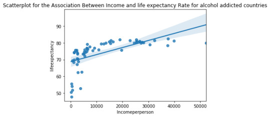
scat1 = seaborn.regplot(x="incomeperperson", y="lifeexpectancy", fit_reg=True,data=sub1) plt.xlabel('Incomeperperson') plt.ylabel('lifeexpectancy') plt.title('Scatterplot for the Association Between Income and life expectancy Rate for non-alcohol addicted countries') print (scat1)

scat2 = seaborn.regplot(x="incomeperperson", y="lifeexpectancy", fit_reg=True, data=sub2) plt.xlabel('Incomeperperson') plt.ylabel('lifeexpectancy') plt.title('Scatterplot for the Association Between Income and life expectancy Rate for alcohol addicted countries') print (scat2)

Output:

Bi-variate graphs:

Discussion:

1) The association between income of a person and life expectancy independent of moderator yielded:

r=0.5953 ----> Positive and moderately strong relationship

p-value= 8.87e-18 ---->Significant

2) The association between income of a person and life expectancy independent for non-alcohol addicted countries.

r=0.508----> Positive and moderately strong relationship

p-value=1.64e-08 ------> Significant

3) The association between income of a person and life expectancy independent for alcohol addicted countries.

r=0.609----> Positive and moderately strong relationship

p-value=1.47e-07 ------> Significant.

Conclusion:

1) Overall, all the three types of analyses are positive and strongly related. So, with or without alcohol addiction association between income and life expectancy are not effected much.

2) By observing both the plots, one can say that parabola would fit the points more effective than straight line.

[varun-data-analysis]

Assignment3- Pearson Correlation

Research Question- Association between Income of a person and type of Alcohol consumer.

Dataset: Gapminder

Null Hypothesis: 1)There is no association between income of a person and quantity of alcohol consumed.

2) There is no association between employment rate of a country and average quantity of alcohol consumed per person.

Alternate Hypothesis: There is an association between them.

Program:

Bivariate scatter plots:

1) scatter plot -1

2) Scatter plot-2

Output:

association between incomeperperson and alcoholconsumption (0.28864262546557856, 0.00019533523307706355) association between employrate and alcoholconsumption (-0.118889517968538, 0.13184952360331226)

Conclusion:

1) r=0.2886-------> Positive but Weak relationship

    p-value= 0.00009 means Significant

r^2=0.083means only a 8% variability van be predicted by one of the known variable.

  So Income per person and alcohol consumption are related but weakly.

2)r=-0.1188--------> Negative and weak relationship

   p-value=0.13>0.05 means insignificant.

So employment and alcohol consumption are not related.

overall, income and alcohol consumption are weakly related whereas employment rate and alcohol consumption are not related they have no association.

[varun-data-analysis]

Assignment-2-chi-square Test

Research Question- Association between Income of a person and type of Alcohol consumer.

Dataset: Gapminder

Null Hypothesis: There is no association between income of a person and type of alcohol consumer.

Alternate Hypothesis: There is an association between them.

Explanatory/Independent Variable: ‘Income_group‘ categorized into four groups

1- < $1000

2- <$12000

3- <$25000

4 - <$105200

Response/Dependent variable:’alcohol_group’ in litres/year categorized into two groups.

0-> 0-8 litres/year->Non-addicted drinker

1->8-25 litres/year-> Addicted drinker

Program:

# -*- coding: utf-8 -*- """ Created on Thu Sep 10 11:54:45 2020

@author: Varun """

import pandas as pd import scipy.stats import seaborn import matplotlib.pyplot as plt import itertools

data_import = pd.read_csv('gapfinder_pds.csv', low_memory=False) data=pd.DataFrame()

data = data_import[['country','incomeperperson', 'alcconsumption', 'employrate']].copy() print("Number of Countries = ", len(data)) #number of observations (rows) print ("Number of Variables =", len(data.columns)) # number of variables (columns)

data['incomeperperson'] = pd.to_numeric(data['incomeperperson'], errors='coerce') data['alcconsumption'] = pd.to_numeric(data['alcconsumption'], errors='coerce') data['employrate'] = pd.to_numeric(data['employrate'], errors='coerce')

labels_income = ['1','2','3','4'] data['income_group'] = pd.cut(data['incomeperperson'], bins=[0,1000,12000,25000,105200], labels=labels_income)

labels_alcohol = ['0','1'] data['alcohol_group'] = pd.cut(data['alcconsumption'], bins=[0,8,25], labels=labels_alcohol)

#Contigency table for observed counts ct1=pd.crosstab(data['alcohol_group'],data['income_group']) print(ct1)

#column percentages colsum=ct1.sum(axis=0) colpct=ct1/colsum print(colpct)

print('chi-sqaure value, p-value and expected values') cs1=scipy.stats.chi2_contingency(ct1) print(cs1)

# set variable types data["income_group"] = data["income_group"].astype('category') # new code for setting variables to numeric: data['alcohol_group'] = pd.to_numeric(data['alcohol_group'], errors='coerce')

seaborn.catplot(x="income_group", y="alcohol_group", data=data, kind="bar", ci=None) plt.xlabel('Income categroies') plt.ylabel('Proportion of highly alcohol addicted people')

# To perform post hoc tests of Berferroni adjustments, good bye to ardous lines of coding for tests using itertools

data['income_group']=pd.to_numeric(data['income_group'],errors='coerce') for pair in itertools.combinations([1,2,3,4],2):    ct=pd.crosstab(data['income_group'].isin(pair), data['alcohol_group'])    print("chi sq test of subcategory: {}".format(pair))    print (scipy.stats.chi2_contingency(ct))

Output:

Conclusion:

Model Interpretation for Chi-Square Tests:

When examining the association between type of alcohol consumer (categorical response) and type of income_group (categorical explanatory), a chi-square test of independence revealed that , those belonging to income_group -4 are more addicted drinkers (77%) next to catergory-3(73%) and least addicted drinkers are in category-1(%). It has chi-square of 36 and p-value of 5.06e-08.The p-value is significant and as it is 4 category explanatory variable I conducted post hoc test of Bonferroni Adjustments.

Model Interpretation for post hoc Chi-Square Test results:

Four categories so adjusted p-value is 0.05/6=0.008.

(1,2)---->chi-square=16.589  p-value=4.639e-05 <<0.008

(1,3)---->chi-square=6.802    p-value= 0.00910 >0.008

(1,4)---->chi-square=4.014    p-value=  0.0451>0.008

(2,3)---->chi-square=5.172    p-value= 0.022951>0.008

(2,4)---->chi-square=8.194    p-value= 0.0042<0.008

(3,4)---->chi-square=23.182   p-value= 1.47e-06<<<0.008

(1,2), (2,4), (3,4) are significant and other are not significant.

Below is the same shown graphically

[varun-data-analysis]

Course2- Assignment1-ANOVA

Research Question- Association between Income of a person and quantity of Alcohol consumption.

Dataset: Gapminder

Null Hypothesis: There is no association between income of a person and quantity of alcohol consumed by him

Alternate Hypothesis: There is an association between them.

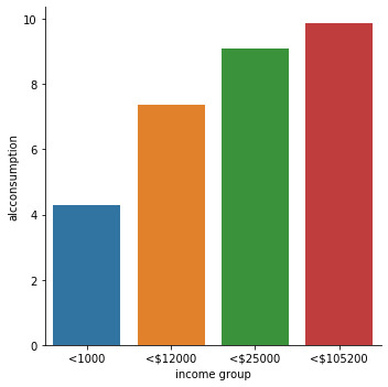
Explanatory/Independent Variable: ‘Incomeperperson‘ categorized into four groups

1- < $1000

2- <$12000

3- <$25000

4 - <$105200

Response/Dependent variable:’alcconsumption’ in litres/year

Program:

Output:

Summary:

Model Interpretation for ANOVA:

When examining the association between quantity of alcohol consumed in liters/year(quantitative response) and income of the person (categorical explanatory), an Analysis of Variance (ANOVA) revealed that among four income groups, 4thcategory-high income reported alcohol consumption  significantly more liters/year (Mean=9.87, s.d. 3.68) compared to those with 1st category- low income (Mean=4.30, s.d. ±4.20), F(3, 175)=9.783, p=5.32e-06.

So, seeing the value of p<<<<<<0.05 we can say that it is significant and we can reject the null hypothesis.

Model Interpretation for post hoc ANOVA results:

Post hoc results generated using Tukey’s Honestly Significant Difference method show 6 possible possible combinations. Out of six, three cases are safe to reject the null hypothesis whereas last three cannot reject null hypothesis.

Careful observation shows that only combinations involving income group-1, the null hypothesis is rejected and in other cases it cannot be. So, least income group is removed null hypothesis cannot be rejected

[varun-data-analysis]

Start of Course 2 in Data Analysis

Course name: Data Analysis Tools

In the first course of Data Management and Visualization, we dealt with descriptive statistics like frequency tables, center and spread and basic visualization like uni-variate and bi-variate graphs.

Now in this course, it is based on Inferential Statistics.

Statistical Hypothesis Testing: Assessing evidence provided by the data in favor or against each hypothesis about population.

Inferential statistics is based on drawing results from means of ‘n’ number of samples.

NULL Hypothesis: There is no relationship between Explanatory and Response variables.

Alternate Hypothesis: There is a relationship between both of them.

Steps in Testing Hypothesis:

1. Specify the null and the alternate hypothesis

2. Choose a Sample

3. Assess the evidence

4. Draw Conclusions.

Other Important topics:

P-value

F-value

Types of statistical Tests:

ANOVA- Analysis of variance

X2- chi-square Test of Independence

r- Pearson correlation coefficient

The first assignment is based on ANOVA

[varun-data-analysis]

Final Assignment - Graphs Visualization

Research Questions-

1. Relationship between Income Per Person and Alcohol Consumption

2. Relationship between Employment rate of a country and Alcohol Consumption

Explanatory/Independent Variables: Income per person,Employment rate

Response/Dependent Variable: Alcohol Consumption

Code:

Output:

Number of Countries =  213 Number of Variables = 4 count       190.000000 mean       8740.966076 std       14262.809083 min         103.775857 25%         748.245151 50%        2553.496056 75%        9379.891166 max      105147.437700 Name: incomeperperson, dtype: float64 count    187.000000 mean       6.689412 std        4.899617 min        0.030000 25%        2.625000 50%        5.920000 75%        9.925000 max       23.010000 Name: alcconsumption, dtype: float64 count    178.000000 mean      58.635955 std       10.519454 min       32.000000 25%       51.225000 50%       58.699999 75%       64.975000 max       83.199997 Name: employrate, dtype: float64 Income per person - 4 categories <1000       54 <$12000     95 <$25000     17 <$105200    24 NaN         23 Name: income_group, dtype: int64

Graphs:

Note: Q-Quantitative

          C- Categorical

Univariate Histograms as my question is relationship between Q-Q

1. Univariate  Q histogram of Income per person:

It show that most of the countries are among Low income group. So, it is skewed to right.

2. Univariate Histogram of Alcohol Consumption:

The trend shows that most of the countries consume lower quantity of alcohol.Skewed to the right distribution.

3. univariate Histogram of Employment rate

Unimodal and symmetric distribution with peak at 50% employment.

Bivariate  Q-Q scatter plots:

1. Scatter plot between Income per person and Alcohol Consumption

2. Scatter plot between Employment rate and alcohol consumption:

Two scatter plots show no signs of any relationship between two plotted variables. It will foolish to draw even the trend line as it is evident from the distributions which are very scattered.

So, let us categorize the explanatory variable and try C-Q bar chart.

Bivariate Categorical to Quantitative Bar charts:

1. Bar chart between Income and Alcohol:

This bar chart is some what revealing which shows that higher income countries consume more alcohol.

2.Bar chart between employment rate and alcohol

This bar chart shows that alcohol consumption of a country does not depend on the employment rate of the country.

Conclusion of the Project:

1. The relationship between income and alcohol consumption are linear and positive. So, Higher the income Higher the consumption of the alcohol.

2. There is no association between employment and alcohol consumption. One cannot become the explanation of the other.

[varun-data-analysis]

Third Assignment

Title:

Association between income per person and average alcohol consumption with or without dependency on average employment rate

Introduction:

People  in countries where average income per person is high are more likely to  have inclination for greater alcohol consumption  although there are other factors(like mental, psychological). We all  know unemployment  rate also has a positive effect on drinking behavior. high  People with  higher income have access to better facilities resulting in higher life  expectancy. The more the money a person has he has more tendency and  option to consume more alcohol and it is also equally true that  unemployed person out of grief and anxiety consumes more alcohol  although the cheaper brands. so my research questions are

Research Question:

Is there an association between average income and alcohol consumption

Is there an association between alcohol consumption and employment rate.

My dataset is GapMinder. This is not a population survey based. It is the data of important parameters of a country like income per person, suicide rate and so on. So, there is no possibility of finding frequency of a certain value of certain category.(example- Income per person of a country is quantitative and   different  countries have diverse value, so even if we do frequency analysis hardly two values are exact, so it is no use) So, I created categorical variable myself and grouped my choice of variables into three categories( like high, medium, low). This is certainly a type of data management ( GROUPING VALUES WITHIN INDIVIDUAL VARIABLE). There is no unknown value in the options for any variable. The answer is either something or left blank(means missing). So, these missing values are already addressed using NAN value in the previous program. So, my point is that data management required for my research is already done to the extent necessary.

What To do!!!?

So I decided to modify my program program so that it is concise and short(like I have used pandas.cut to categorise, now, i will use pandas.qcut). And also to have some fun in learning the operations taught in this week which may not be much relevant or important to the problem but make me learn (which is exactly why we are here!!! ;) )

Program:

# -*- coding: utf-8 -*- """ Created on Tue Sep  1 13:59:29 2020@author: Varun """import pandas as pddata_import = pd.read_csv('gapfinder_pds.csv', low_memory=False) data=pd.DataFrame()data = data_import[['country','incomeperperson', 'alcconsumption', 'employrate']].copy() print("Number of Countries = ", len(data)) #number of observations (rows) print ("Number of Variables =", len(data.columns)) # number of variables (columns)data['incomeperperson'] = pd.to_numeric(data['incomeperperson'], errors='coerce') data['alcconsumption'] = pd.to_numeric(data['alcconsumption'], errors='coerce') data['employrate'] = pd.to_numeric(data['employrate'], errors='coerce')# Grouping values with in Individual Variablelabels_income = ['1=0%tile','2=25%tile','3=50%tile','4=75%tile'] data['income_group'] = pd.qcut(data['incomeperperson'], 4, labels=labels_income)print ('Income per person - 4 categories') c1 = data['income_group'].value_counts(sort=False,dropna=False) print (c1)print ('percentages for Income per person') p1 = data['income_group'].value_counts(sort=False,dropna=False, normalize=True) print (p1)labels_alcohol = ['1=0%tile','2=25%tile','3=50%tile','4=75%tile'] data['alcohol_group'] = pd.cut(data['alcconsumption'], 4, labels=labels_alcohol)print (' "alcconsumption" quantity consumed per person- 4 categories') c2 = data['alcohol_group'].value_counts(sort=False,dropna=False) print(c2)print( 'percentages for "alcconsumption" quantity consumed per person') p2 = data['alcohol_group'].value_counts(sort=False,dropna=False, normalize=True) print (p2)labels_employ = ['1=0%tile','2=25%tile','3=50%tile','4=75%tile'] data['employ_group'] = pd.cut(data['employrate'], 4, labels=labels_employ) print ('counts for employment rate - 4 categories') c3 = data['employ_group'].value_counts(sort=False,dropna=False) print(c3)print ('percentages for employment rate - 4 categories') p3 = data['employ_group'].value_counts(sort=False,dropna=False, normalize=True) print (p3)#secondary variable multiplying the employment rate and the income per person data['total_employees_income_of_country_in_Million$']=data['incomeperperson'] * data['employrate']/(1e+6) print(data[['country', 'total_employees_income_of_country_in_Million$']].head(25))data['total_income_group'] = pd.cut(data['total_employees_income_of_country_in_Million$'], 4, labels=labels_employ) print ('total employees income of country in Million$ - 4 categories') c4 = data['total_income_group'].value_counts(sort=False,dropna=False) print(c4)print ('percentages total employees income of country in Million$ - 4 categories') p4 = data['total_income_group'].value_counts(sort=False,dropna=False, normalize=True) print (p4)

Output:

Number of Countries =  213 Number of Variables = 4 Income per person - 4 categories 1=0%tile     48 2=25%tile    47 3=50%tile    47 4=75%tile    48 NaN          23 Name: income_group, dtype: int64 percentages for Income per person 1=0%tile     0.225352 2=25%tile    0.220657 3=50%tile    0.220657 4=75%tile    0.225352 NaN          0.107981 Name: income_group, dtype: float64 "alcconsumption" quantity consumed per person- 4 categories 1=0%tile     90 2=25%tile    64 3=50%tile    29 4=75%tile     4 NaN          26 Name: alcohol_group, dtype: int64 percentages for "alcconsumption" quantity consumed per person 1=0%tile     0.422535 2=25%tile    0.300469 3=50%tile    0.136150 4=75%tile    0.018779 NaN          0.122066 Name: alcohol_group, dtype: float64 counts for employment rate - 4 categories 1=0%tile     18 2=25%tile    64 3=50%tile    69 4=75%tile    27 NaN          35 Name: employ_group, dtype: int64 percentages for employment rate - 4 categories 1=0%tile     0.084507 2=25%tile    0.300469 3=50%tile    0.323944 4=75%tile    0.126761 NaN          0.164319 Name: employ_group, dtype: float64 total employees income of country in Million$ - 4 categories 1=0%tile     133 2=25%tile     13 3=50%tile     12 4=75%tile      8 NaN           47 Name: total_income_group, dtype: int64 percentages total employees income of country in Million$ - 4 categories 1=0%tile     0.624413 2=25%tile    0.061033 3=50%tile    0.056338 4=75%tile    0.037559 NaN          0.220657 Name: total_income_group, dtype: float64

Summary:

1.  Presence of missing data- addressed using NAN value

2.  Coding in valid data and re-coding values-  Not possible in my dataset as there is no such data(mostly there are found in surveys)

3. Creating Secondary variable -Yes, a new variable is created multiplying “employment rate” and “income per person”

4. Grouping Values within Individual variables - Yes, three such variables are grouped.

5. Discussion of Important Points-

   Based on quartile groping of all four variables,

- Income group- All groups are equally sized i.e, around 22% and remaining is missing data

- Alcohol_group- First two groups i.e, first 50% is dominating with 72%

- Employment group- middle two groups i.e, 25-75% are dominating with 63%

[varun-data-analysis]

Second Assignment

1Title:

Association between income per person and average alcohol consumption with or without dependency on average employment rate

Introduction:

People in countries where average income per person is high are more likely to have inclination for greater alcohol consumption although there are other factors(like mental, psychological). We all know unemployment rate also has a positive effect on drinking behavior. high  People with higher income have access to better facilities resulting in higher life expectancy. The more the money a person has he has more tendency and option to consume more alcohol and it is also equally true that unemployed person out of grief and anxiety consumes more alcohol although the cheaper brands. so my research questions are

Research Question:

Is there an association between average income and alcohol consumption

Is there an association between alcohol consumption and employment rate.

I have created a categorical variables(one each for income,employment, alcohol consumption) in gap minder to analyze data statistically as done in NESARC data file.

Income_group-low(income<$1025), medium($1025<income<$25000), high($25000<income<$110000)

alcohol_group-low(<=5 liters/year ), average(>5 liters/year and ,=15 liters/year ), high(>15 liters/year)

Employ_group- low(<=32%), average(>32% and<=50%) , high(>50%)

  All the classification and limits of the groups are based on some research and personal judgement keeping in view the data available.

  Creating Categorical variables in Python is tedious and difficult task but eventually achieved after long search for attributes and objects of Pandas and so many iterations.

Program:

As the program is lengthy in python I have uploaded it in another post for which the link is https://varun-data-analysis.tumblr.com/post/627783146358915072/first-program-in-python-in-data-analysis

Output:

Nan= no information is available

Number of Countries =  213 Number of Variables = 4

Frequency Table 1:

counts for "income per person" in countries based on high medium and low income, high-income       54 medium-income    112 low-income        24 NaN               23 Name: income_group, dtype: int64 percentages for  countries based on developed,developing and under-developed high-income      0.253521 medium-income    0.525822 low-income       0.112676 NaN              0.107981 Name: income_group, dtype: float64

Frequency Table 2:

counts for "alcconsumption" quantity consumed per person low        80 average    95 high       12 NaN        26 Name: alcohol_group, dtype: int64 percentages for "alcconsumption" quantity consumed per person low        0.375587 average    0.446009 high       0.056338 NaN        0.122066 Name: alcohol_group, dtype: float64

Frequency Table 3:

counts for employment rate low         37 average    114 high        27 NaN         35 Name: employ_group, dtype: int64 percentages for employment rate low        0.173709 average    0.535211 high       0.126761 NaN        0.164319 Name: employ_group, dtype: float64

Summary:

Variables income per person, alcohol consumption, employment rate are categorized to carry out frequency calculations. 52% countries fall under medium income group where as 25% and 11% under high and low income respectively.Similar correlation is observed in alcohol consumption and employment rate too, 44% which is the highest among the group fall under average consumers of alcohol and 53% of the countries are moderately employed. The missing data is also accounted for using Nan, 10, 12, 16 % data is missing in income,alcohol and employment variables respectively.

[varun-data-analysis]

First Program in Python in Data Analysis

""" Created on Sun Aug 23 16:27:43 2020

@author: Varun """

import pandas as pd

data_import = pd.read_csv('gapfinder_pds.csv', low_memory=False) data=pd.DataFrame()

data = data_import[['country','incomeperperson', 'alcconsumption', 'employrate']].copy() print("Number of Countries = ", len(data)) #number of observations (rows) print ("Number of Variables =", len(data.columns)) # number of variables (columns)

data['incomeperperson'] = pd.to_numeric(data['incomeperperson'], errors='coerce') data['alcconsumption'] = pd.to_numeric(data['alcconsumption'], errors='coerce') data['employrate'] = pd.to_numeric(data['employrate'], errors='coerce') #ADDING MORE DESCRIPTIVE TITLES

labels_income = ['high-income','medium-income','low-income'] data['income_group'] = pd.cut(data['incomeperperson'], bins=[0,1025,25000,110000], right=False, labels=labels_income)

print ('counts for "income per person" in countries based on high medium and low income,') c1 = data['income_group'].value_counts(sort=False,dropna=False) print (c1)

print ('percentages for  countries based on developed,developing and under-developed') p1 = data['income_group'].value_counts(sort=False,dropna=False, normalize=True) print (p1)

labels_alcohol = ['low','average','high'] data['alcohol_group'] = pd.cut(data['alcconsumption'], bins=[0,5,15,25], right=False, labels=labels_alcohol)

print ('counts for "alcconsumption" quantity consumed per person') c2 = data['alcohol_group'].value_counts(sort=False,dropna=False) print(c2)

print( 'percentages for "alcconsumption" quantity consumed per person') p2 = data['alcohol_group'].value_counts(sort=False,dropna=False, normalize=True) print (p2)

labels_employ = ['low','average','high'] data['employ_group'] = pd.cut(data['employrate'], bins=[0,50,70,100], right=False, labels=labels_employ) print ('counts for employment rate') c3 = data['employ_group'].value_counts(sort=False,dropna=False) print(c3)

print ('percentages for employment rate') p3 = data['employ_group'].value_counts(sort=False,dropna=False, normalize=True) print (p3) print(data)

[varun-data-analysis]

My First Assignment-choosing a research question.

I went through all the code books provided in the course. I choose to take Gap Finder to frame my research question. After going through the Gap Finder Code book I found my interest in the alcohol consumption and Internet usage rate. Eventually I narrowed it down to Alcohol Consumption.

Usually alcohol consumed by a person depends on many factors like Socio-economic status, employment status, Housing status, Religion, age, mental status and so on. During my graduation, I found some of my friends got addicted to alcohol which mainly kick started as soon as they got employment. They felt a sense of relief as they landed in a job and that none can stop them as they need stretch one’s hands for money to buy it. So, it triggered in my mind that income of a person very much defines whether one fall to this addiction or not. So my second variable is Per capita Income of a person.A study of association between alcohol consumption and Per capita Income is worth a shot.

Literature Review

1. World Health Organization (WHO) comes handy in these cases. In Global Status report on alcohol and health 2018, they categorized countries into High, middle and low income countries. It is reported that High income countries consume more alcohol compared to middle and low.

source: Table 3.11

https://apps.who.int/iris/bitstream/handle/10665/274603/9789241565639-eng.pdf?ua=1

2. An article by Our World in Data, shows a chart describing association between Alcohol consumption and  GDP Per capita of different countries. The trend is  found to be linear and positive with some exception in Asian countries.

Source: World Bank- World Development Indicators.(2016)

https://ourworldindata.org/grapher/alcohol-consumption-vs-gdp-per-capita

Hypothesis:

After going through Literature, I predict that the association will be linear and positive. The Asian countries will be out of trend with more distributed like a bell-shaped curve. It means alcohol consumption is high in moderate income countries and low in rich and poor countries of Asia.

[varun-data-analysis]

Here Begins my Journey

Hello friends,

I am your dearest friend, Varun Vidiyala. Data analyst and data scientist are the top seeking jobs in this era. So, I thought like why shouldn’t I have the skill sets required for those profiles.

I started searching online for skills required. The top most skills required is Statistics and Programming. I have a fair understanding of Statistics in my graduation. So, I researched for Programming language required which pointed at two languages- SAS and Python. Owing to the universal acceptability and diverse applications of Python I did a basic course in Python. Hurray!!!! It is my internal feeling inside me after completing my course in Python. But the job is not done yet as the statistics used and application of programming is different in data analysis. It needs some supervise learning through Courses to acquire acquaintance with data sampling, cleaning, algorithms, regressing analysis etc..etc..etc..

I enrolled in Data Management and Visualization offered by Wesleyan University through Coursera.

It is a nice course. Learning through application is the motto of the course. For further updates regarding my journey through data analysis.

Stay Tuned !!!!!