zeenahawamdeh

[zeenahawamdeh]

Milestone Assignment 3: Preliminary Results

I don’t know about you, but I’m pretty much ready for this to be over…

I’m going to post screen shots of my current results here, so you can see I’ve been working. In the final report, I’ll be improving upon the presentation, making sure the layout, wording and all the rest is in good shape. The numbers are all there though, so enjoy…

[zeenahawamdeh]

Capstone Milestone Assignment2: Methods

Please note:

After wasting days, ‘massaging’ data and yet more days, trying to get any sort of value out of my National Weather Service (NWS) dataset, I reluctantly decided to abandon it, in favor of my own data. I’ve worked with data for a good 30 years. So far, I’ve been far from impressed with either dataset I’ve used on this course. Either there is not enough data, lengthwise for real comparison, or the data is more a collection of partial, un-related pieces of information. I found the latter to be the case with NWS. It was just a tumbleweed of data. A whole collection of somewhat inconsistent data (with crazy outliers), that adhered to the dataset, as it tumbled around. Perhaps with hindsight, I would have approached the dataset differently. However, having coded an entire solution (that pretty much showed nothing useful), I decided to use some data that I’m more familiar with.

Test Scores

I apologize for being somewhat vague about my dataset. It is real data and has not been modified in any way. Because it is real and part of a somewhat sensitive nature, I have decided to keep the description as simple as possible. There is nothing personally identifiable in it, but out of respect to the provider, I am going to not go into specifics.

Sample

My data is based Test Scores (n=4907) for an exam. It consists of results acquired over a period of 3 years (2019-2021).

Measures

I am interested in what may have influenced test scores. I have decided to consider if any of the following factors could influence them:

Gender (1)– whether the person taking the test was Male or Female.

The takers Standing (2), professionally – i.e. is there anything about them that might have damaged their professional reputation (perhaps they have been in legal trouble, for example).

How many other Different Types of Exam (3), the taker of this exam has undertaken. Some people will be multi-disciplinary and take more than one type of exam.

Whether the person tested was Educated in the US (4), or overseas.

The Day (5) the person tested took the exam. Note, a test is administered multiple times, over several days. Day 3, for example, would be the 3rd day in a testing cycle that the test was administered. It could be a Wednesday, if the exam cycle started on a Monday. If the exam cycle started on a Wednesday, Day 3 would be a Friday. I would like to know if an exam possibly gets easier or harder, the more times it is administered.

The Total Score (6) given to the person tested for their exam.

The Age (7) of the person being tested, at the time of the exam.

The Number of Times (8)the person has taken this test. Note, 1 attempt means the person took the test and either passed (and will never re-take) or failed (and will have to repeat the test).

Analyses

In order to understand the predictors of the Exam Scores response variable, distribution of the explanatory variables were determined by calculating the frequency of categorial variable and mean, standard deviation, minimum and maximum values for the quantitative variables.

Scatter and box plots were created to assist with the analysis.

In order to check the bivariate associations between the explanatory variables and the Scores response variable, Pearson and Analysis of Variance (ANOVA) calculations were also performed upon the Quantitative and Categorical Explanatory variables, respectively.

Predicting the best subset of variables that may predict exam scores was performed by using Lasso regression analysis. A random sample training dataset was employed, consisting of 65% of the overall sample (N=3190), along with the corresponding random sample test dataset (N=1717). Explanatory variables were standardized (with a mean set to 0 and 1 for standard deviation). Finally, K-fold analysis was used to perform cross-validation, with 9 folds specified. Finally, the cross validation mean-squared error deviation identified the best choice of predictor variables. Predictive accuracy was assessed from analyzing the mean-squared error rate from the training prediction results, after applied to the test dataset observations.

[zeenahawamdeh]

Capstone Projest - Week 1

Capstone Project Title

The Association between climate change and economic indicators in low, medium and high income countries.

Introduction and motivation to research the project

The purpose of this research is to measure the best predictors of a country’s climate change contribution from several economic indicators such as energy consumption, export and import of goods and services, urbanization, industry and gross domestic product (GDP) per capita.

 We live in an age where the planetary boundaries (such as climate change, ocean acidification, ozone depletion, heavy agriculture loading of nitrogen and phosphorus, overuse of flesh water resources, and biodiversity loss) are getting stressed in addition to increasing poverty in many parts of the world. Global economic activities have pushed the subject of climate change and sustainability to the main stream where individuals, businesses and governments are facing increasing pressure to take action to curve greenhouse gas emissions in order to avoid catastrophic impacts from global warming.

The starting point of tackling this problem of the commons is to measure and understand which economic predictors are associated most with climate change (co2 emissions) and thereby developing adaptation and mitigation strategies towards a sustainable future of our planet.

 I am currently developing new skills in climate change policy, accounting and sustainability reporting. As a native of West Africa and currently living in Canada (North America), I have chosen three groups of countries represented as follows:

a) Low income countries: 15 member Ecowas countries located around the equator and within the sub-Saharan region where climate change impact is predicted to be severe. Investigating the relationship between economic activities and climate change will help those countries to channel their scarce resources to help develop resilience strategies.

b) Middle income countries: 26 countries including Mexico (North America), who are not spared from climate change impacts. I am hoping this study will add to the growing need for these countries to balance between economic activity and emission control and

c) High income country: 26 countries including Canada, which have become a model for other countries in terms of industrialization. I hope this study will contribute to the glowing need to develop energy efficiency technologies and a shift towards renewable energy.

 Dataset Information

I am using the world bank dataset provided by the course. Firstly, the dataset will be cleaned up to include 67 countries representing the 3 income levels (out of the 198 countries provided by the dataset). Secondly, reductant columns from the dataset will be deleted so that the study can be focussed on the indicator variables mentioned. Finally, A series of test including descriptive statistics, scatter plots, Pearson correlation and regression analysis will be conducted to complete the project.

 In summary, prediction of a moderate to high relationship between economic activities and climate change will move governments of these countries towards a more proactive action on climate and sustainability.

[zeenahawamdeh]

Running a k-means Cluster Analysis

A k-means cluster analysis was conducted to identify underlying subgroups of lifestyles/habits based on 14 variables. Clustering variables included quantitative variables measuring

INCOME PER PERSON, ALC CONSUMPTION, ARMED FORCES RATE, BREAST CANCER PER 100TH. CO2 EMISSIONS, FEMALE EMPLOYRATE, HIV RATE, INTERNET USE RATE, OIL PER PERSON, POLITY SCORE, ELECTRIC PER PERSON, SUICIDE PER 100TH, EMPLOY RATE, URBAN RATE

All clustering variables were standardized to have a mean of 0 and a standard deviation of 1.

Data were randomly split into a training set that included 70% of the observations (N=39) and a test set that included 30% of the observations (N=17). A series of k-means cluster analyses were conducted on the training data specifying k=1-9 clusters, using Euclidean distance. The variance in the clustering variables that was accounted for by the clusters (r-square) was plotted for each of the nine cluster solutions in an elbow curve to provide guidance for choosing the number of clusters to interpret.

Figure 1. Elbow curve of r-square values for the nine cluster solutions

The elbow curve was inconclusive, suggesting that the 2 and 4 cluster solutions might be interpreted. The results below are for an interpretation of the 4-cluster solution.

Canonical discriminant analyses was used to reduce the 14 clustering variable down a few variables that accounted for most of the variance in the clustering variables. A scatterplot of the first two canonical variables by cluster (Figure 2 shown below) indicated that the observations in clusters 1 through 4 were distinct and did not overlap with the other clusters. Observations in cluster 4 or deep red were spread out more than the other clusters, showing high within cluster variance.

Figure 2. Plot of the first two canonical variables for the clustering variables by cluster.

The means on the clustering variables showed that, compared to the other clusters, cluster 1 had highest HIV Rate and cluster 4 had the income per person, highest urban rate, employ rate, oil per person, electric per person and internet use rate. All in all cluster 4 had a better life and thus higher life expectancy was evident. And higher HIV RATE points to lower life expectancy.

In order to externally validate the clusters, an Analysis of Variance (ANOVA) was conducting to test for significant differences between the clusters on LIFE EXPECTANCY. A tukey test was used for post hoc comparisons between the clusters. The tukey post hoc comparisons showed significant differences between clusters on, LIFE EXPECTANCY with the exception that clusters 2 and 3 were not significantly different from each other. People in cluster 4 had the highest LIFE EXPECTANCY (mean=78.06, sd=4.6), and cluster 1 had the lowest LIFE EXPECTANCY (mean=68.25, sd=10.31).

[zeenahawamdeh]

Running a Lasso Regression Analysis

Data were randomly split into a training set that included 70% of the observations (N=37,758) and a test set that included 30% of the observations (N=16,182). The least angle regression algorithm with k=10 fold cross validation was used to estimate the lasso regression model in the training set, and the model was validated using the test set. The change in the cross validation average (mean) squared error at each step was used to identify the best subset of predictor variables.

[zeenahawamdeh]

Peer-graded Assignment: Running a Random Forest

Machine Learning for Data Analysis - HPForest

Second exercise of the course.

I have used the example of the course modifying the level of target TREG1 to "interval":

PROC HPFOREST; target TREG1/level=interval;

The results of the program are next:

[zeenahawamdeh]

Running a Classification Tree

Decision trees

DATA base; set mydatatree; run;

proc sort; by ID;

ods graphics on; proc hpsplit seed=15531; class TREG1 sex latin white income vstore vpharmacy bmeat bveg bfruit bmilk; model TREG1 =sex latin white income alcevr1 ALCPROBS1 vstore vpharmacy bmeat bveg bfruit bmilk; grow entropy; prune costcomplexity;

run;

PROC IMPORT DATAFILE= "data; sheet = "Sheet1"; getnames=yes; RUN;

DATA base; set mydatatree;

republican=1; if dem=1 then republican=2; run;

proc sort; by ID;

ods graphics on; run; proc hpsplit data=base;

class republican Age MW S W urban married female white hisp college hhsize inc minors employed ; model republican = Age MW S W urban married female white hisp college hhsize inc minors employed; grow entropy; prune costcomplexity;

run;

[zeenahawamdeh]

Regression Modeling in Practice Week 4

When building a logistic regression, I divided the variable responsible for the rate of death of 100,000 people into two categories. First of all, there were data that included cases of a smaller number of 9, the second included those that included a level greater than or equal to 9.

However, the results are not representative enough. We propose to trace and prosecute, but it is not possible to talk about the alleged relationships. Adding extended explanatory variable is only leading to accept the null hypothesis on all variables.

Each added variable added is not significant at the event level per 100,000 people.

Below are the results

[zeenahawamdeh]

Week 2. Basic Linear Regression Model

Research question: is there an association between major depression and the frequency with which young adults ages 18-25 drink?

Program:

import numpy import pandas import statsmodels.api as sm import seaborn import statsmodels.formula.api as smf from matplotlib import pyplot as plt

Bug fix for display formats to avoid run time errors

pandas.set_option('display.float_format', lambda x:'%.2f'%x)

Call in data set

data = pandas.read_csv('nesarc_pds.csv', low_memory=False)

DATA MANAGEMENT

Set the variables that will be used for the study to numeric

data['MAJORDEPLIFE'] = pandas.to_numeric(data['MAJORDEPLIFE'], errors='coerce') data['AGE'] =pandas.to_numeric(data['AGE'], errors='coerce') data['S2AQ3'] =pandas.to_numeric(data['S2AQ3'], errors='coerce') data['S2AQ15R1'] =pandas.to_numeric(data['S2AQ15R1'], errors='coerce') data['S2AQ8A'] =pandas.to_numeric(data['S2AQ8A'], errors='coerce')

Recode all the unknown values to missing values

data['S2AQ15R1']=data['S2AQ15R1'].replace(999, numpy.nan) data['S2AQ8A']=data['S2AQ8A'].replace(99, numpy.nan)

Make sure the categorical explanatory variable is code 0 to "no" and 1 to "yes"

chk1 = data['MAJORDEPLIFE'].value_counts(sort=False) print (chk1)

Output:

0: 35254 1: 7839 Name: MAJORDEPLIFE, dtype: int64

Define a subset only considering participants from 18 to 25 years old who drank at least 1 alcoholic drink in the past 12 months and who drank their last drink in the last month

sub1=data[(data['AGE']<=25) & (data['S2AQ3']==1) & (data['S2AQ15R1']<=1)]

Recode 1,2 to 0,1 for summing after recoding values of 9 to missing values

recode1 = {1: 1, 2: 0} sub1['S2AQ3']=sub1['S2AQ3'].replace(9, numpy.nan) sub1['S2AQ3']= sub1['S2AQ3'].map(recode1)

chk2 = sub1['S2AQ3'].value_counts(sort=False) print (chk2)

Output:

1: 3032 Name: S2AQ3, dtype: int64

END DATA MANAGEMENT

CATEGORICAL EXPLANATORY VARIABLES

Research question: is there an association between major depression and the frequency with which young adults ages 18-25 drink?

Major depression: binary categorical explanatory variable

Drinking frequency: quantitative response variable

reg1 = smf.ols('S2AQ8A ~ MAJORDEPLIFE', data=sub1).fit() print (reg1.summary())

Listwise deletion for calculating means for regression model observations

sub2 = sub1[['S2AQ8A', 'MAJORDEPLIFE']].dropna()

Output:

Group means and standard deviations

print ("Mean") ds1 = sub2.groupby('MAJORDEPLIFE').mean() print (ds1) print ("Standard deviation") ds2 = sub2.groupby('MAJORDEPLIFE').std() print (ds2)

Output:

Mean S2AQ8A MAJORDEPLIFE 0: 5.54 1: 5.58 Standard deviation S2AQ8A MAJORDEPLIFE 0: 2.23 1: 2.34

Bivariate bar graph

seaborn.catplot(x="MAJORDEPLIFE", y="S2AQ8A", data=sub1, kind="bar", ci=None) plt.xlabel('Major Life Depression') plt.ylabel('Mean Drinking Frequency')

Output:

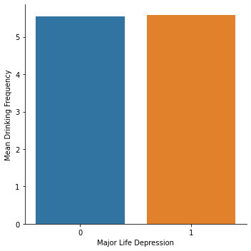
Interpretation of OLS Regression Results:

The results of the linear regression model indicate that the parameter estimate for lifetime major depression is 0.043, that is, it is positively associated with the frequency with which young adults ages 18-25 drink. However, lifetime major depression has a very high p-value: 0.667 > 0.05. This means that the parameter estimate for lifetime major depression is not significantly different from 0.

The model shows that it does not matter if a young adult ages 18-25 who drank at least 1 alcoholic drink in the last 12 months and who had their last drink in the last month suffers or not from lifetime major depression. Lifetime major depression will not determine significantly whether the participant drinks more frequently or not. Participants from the sample, whether depressed or not, are expected to drink 2 to 3 times a month, on average.

[zeenahawamdeh]

Regression Modeling in Practice: Assign-01 - step 3

 a) Describe what your explanatory and response variables measured. The list below are the explanatory and response variable as potential candidates, selected for my research.

From section 2 under daily activities the following data elements are potential candidates to the explanatory variable.

H1DA1 (House Work/Chores) H1DA2 {Hobbies} H1DA3 {TV/Video Games} H1DA4 {Physical Activity -> biking…roller blading} H1DA5 {Active Sports -> Soccer, baseball} H1DA6 {Exercise}

From section 10 under feeling scale the following data elements are potential candidates for reponse variable.

H1FS1 {bothered by things that usually don’t bother you.} H1FS4 {feel good as other people} H1FS6 {feel Depressed} H1FS7 {Feel too tired} H1FS9 {feel life is a failure} H1FS11 {feel happy} H1FS14 {feel people were unfriendly to you} H1FS15 {enjoyed life} H1FS16 {feel sad} H1FS17 {felt that people disliked you} H1FS18 {was hard to get started doing things} H1FS19 {felt life was not worth living}

b) Describe the response scales for your explanatory and response variables. The explanatory and the response variables are both categorical. 

c) Describe how you managed your explanatory and response variables. Since, all the selected data elements for explanatory and response variables are categorical, the survey had 4 options to indicate their degree or frequency or measure as a response. There were two more options provided for the respondent to refuse to answer or to claim unawareness. For the latter two options, I used it as missing data.

[zeenahawamdeh]

Regression Modeling in Practice: Assign-01 - step 2

Step 2: Describe the procedures that were used to collect the data.

 a) Report the study design that generated that data (for example: data reporting, surveys, observation, experiment). The study design that was used to generate the data was survey (questionnaires) filled in by an In-Home interviewer. 

b) Describe the original purpose of the data collection. The purpose of this longitudinal data collection is to study the environmental impacts and the outcome of the adolescent students.

 c) Describe how the data were collected. The data was collected by an interviewer.  He recorded the answers of the response of the respondents

 d) Report when the data were collected. The wave1 Data was collected between 1994 and 1977.  This wave1 holds data of my research interest.

 e) Report where the data were collected? The wave1 data was collected via home interview from a fixed set of questions.

[zeenahawamdeh]

Regression Modeling in Practice: Assign-01

Step 1:

a) Describe the study population (who or what was studied).

The sample population is students from high school in United States of America. The focus of this study was on student adolescents.  The data is collected in 5 waves from the same sample set and each wave indicates a maturing phase of the individual. 

b) Report the level of analysis studied (individual, group, or aggregate).

Each adolescents student was studied individually through self-reporting and through interview.

c) Report the number of observations in the data set. There were 6504 adolescent students participated in the study.

 d) Describe your data analytic sample (the sample you are using for your analyses). The following data elements are potential candidates for my research. Each data elements were part of the wave 1 research and it was collected via in-home interview.

 From section 2 under daily activities the following data elements attribute to the explanatory variable.

H1DA1 (House Work/Chores) H1DA2 {Hobbies} H1DA3 {TV/Video Games} H1DA4 {Physical Activity -> biking…roller blading} H1DA5 {Active Sports -> Soccer, baseball} H1DA6 {Exercise}

From section 10 under feeling scale the followingH1FS1 {bothered by things that usually don’t bother you.}

H1FS4 {feel good as other people} H1FS6 {feel Depressed} H1FS7 {Feel too tired} H1FS9 {feel life is a failure} H1FS11 {feel happy} H1FS14 {feel people were unfriendly to you} H1FS15 {enjoyed life} H1FS16 {feel sad} H1FS17 {felt that people disliked you} H1FS18 {was hard to get started doing things} H1FS19 {felt life was not worth living}

[zeenahawamdeh]

Data Analysis Tools - Week 04

import pandas

import numpy

import scipy.stats

import seaborn

import matplotlib.pyplot as plt

data = pandas.read_csv(‘gapminder.csv’, low_memory=False)

data['urbanrate’] = data['urbanrate’].convert_objects(convert_numeric=True)

data['incomeperperson’] = data['incomeperperson’].convert_objects(convert_numeric=True)

data['internetuserate’] = data['internetuserate’].convert_objects(convert_numeric=True)

data['incomeperperson’]=data['incomeperperson’].replace(’ ’, numpy.nan)

data_clean=data.dropna()

print (scipy.stats.pearsonr(data_clean['urbanrate’], data_clean['internetuserate’]))

def incomegrp (row):

   if row['incomeperperson’] <= 744.239:

      return 1

   elif row['incomeperperson’] <= 9425.326 :

      return 2

   elif row['incomeperperson’] > 9425.326:

      return 3

data_clean['incomegrp’] = data_clean.apply (lambda row: incomegrp (row),axis=1)

chk1 = data_clean['incomegrp’].value_counts(sort=False, dropna=False)

print(chk1)

sub1=data_clean[(data_clean['incomegrp’]== 1)]

sub2=data_clean[(data_clean['incomegrp’]== 2)]

sub3=data_clean[(data_clean['incomegrp’]== 3)]

print ('association between urbanrate and internetuserate for LOW income countries’)

print (scipy.stats.pearsonr(sub1['urbanrate’], sub1['internetuserate’]))

print (’       ’)

print ('association between urbanrate and internetuserate for MIDDLE income countries’)

print (scipy.stats.pearsonr(sub2['urbanrate’], sub2['internetuserate’]))

print (’       ’)

print ('association between urbanrate and internetuserate for HIGH income countries’)

print (scipy.stats.pearsonr(sub3['urbanrate’], sub3['internetuserate’]))

#%%

scat1 = seaborn.regplot(x=“urbanrate”, y=“internetuserate”, data=sub1)

plt.xlabel('Urban Rate’)

plt.ylabel('Internet Use Rate’)

plt.title('Scatterplot for the Association Between Urban Rate and Internet Use Rate for LOW income countries’)

print (scat1)

#%%

scat2 = seaborn.regplot(x=“urbanrate”, y=“internetuserate”, fit_reg=False, data=sub2)

plt.xlabel('Urban Rate’)

plt.ylabel('Internet Use Rate’)

plt.title('Scatterplot for the Association Between Urban Rate and Internet Use Rate for MIDDLE income countries’)

print (scat2)

#%%

scat3 = seaborn.regplot(x=“urbanrate”, y=“internetuserate”, data=sub3)

plt.xlabel('Urban Rate’)

plt.ylabel('Internet Use Rate’)

plt.title('Scatterplot for the Association Between Urban Rate and Internet Use Rate for HIGH income countries’)

print (scat3)

[zeenahawamdeh]

Data Analysis Tools - WEEK 03

Summary :Research Project :

I am interested in finding the relationship between Urban Rate, Life Expectancy and C02 Emissions.

Now a days, more and more people are now moving to urban cities in hopes of Jobs and better life. But do they actually get that ? Or they end up in derogating their life quality and reduce the Life Expectancy of their children and next generations!

Code Book :

co2emissions : Total amount of CO2 emission in metric tons since 1751

lifeexpectancy : The average number of years a newborn child would live if current mortality patterns were to stay the same.

urbanrate :Percentage of total people living in urban areas.

Analysis program :

Output of the program :

Summary :

Pearson Correlation:

Value of r observed = 0.621 [Strong, Positive Relation]

P value = 1.091e-20 [Very small, < 0.05]

So,  using the value of r and visually interpreting the scatter-plot, we can say that life expectancy and urban rate are related. They have strong positive relationship.

Moreover if we square the value of r its value is 0.38, ie r^2 = 0.38.

So we can predict 38% of variability we will see in the urban rate.

Note : Pearson Correlation does not need any post hoc test.

[zeenahawamdeh]

Running a Chi-Square Test of Independence - Nearc_pds

import pandas import numpy import scipy.stats import seaborn import matplotlib.pyplot as plt

data = pandas.read_csv(‘nesarc.csv’, low_memory=False)

“”“ setting variables you will be working with to numeric 10/29/15 note that the code is different from what you see in the videos A new version of pandas was released that is phasing out the convert_objects(convert_numeric=True) It still works for now, but it is recommended that the pandas.to_numeric function be used instead ”“”

“”“ old code: data['TAB12MDX’] = data['TAB12MDX’].convert_objects(convert_numeric=True) data['CHECK321’] = data['CHECK321’].convert_objects(convert_numeric=True) data['S3AQ3B1’] = data['S3AQ3B1’].convert_objects(convert_numeric=True) data['S3AQ3C1’] = data['S3AQ3C1’].convert_objects(convert_numeric=True) data['AGE’] = data['AGE’].convert_objects(convert_numeric=True) ”“”

new code setting variables you will be working with to numeric

data['TAB12MDX’] = pandas.to_numeric(data['TAB12MDX’], errors='coerce’) data['CHECK321’] = pandas.to_numeric(data['CHECK321’], errors='coerce’) data['S3AQ3B1’] = pandas.to_numeric(data['S3AQ3B1’], errors='coerce’) data['S3AQ3C1’] = pandas.to_numeric(data['S3AQ3C1’], errors='coerce’) data['AGE’] = pandas.to_numeric(data['AGE’], errors='coerce’)

subset data to young adults age 18 to 25 who have smoked in the past 12 months

sub1=data[(data['AGE’]>=18) & (data['AGE’]<=25) & (data['CHECK321’]==1)]

make a copy of my new subsetted data

sub2 = sub1.copy()

recode missing values to python missing (NaN)

sub2['S3AQ3B1’]=sub2['S3AQ3B1’].replace(9, numpy.nan) sub2['S3AQ3C1’]=sub2['S3AQ3C1’].replace(99, numpy.nan)

recoding values for S3AQ3B1 into a new variable, USFREQMO

recode1 = {1: 30, 2: 22, 3: 14, 4: 6, 5: 2.5, 6: 1} sub2['USFREQMO’]= sub2['S3AQ3B1’].map(recode1)

contingency table of observed counts

ct1=pandas.crosstab(sub2['TAB12MDX’], sub2['USFREQMO’]) print (ct1)

column percentages

colsum=ct1.sum(axis=0) colpct=ct1/colsum print(colpct)

chi-square

print ('chi-square value, p value, expected counts’) cs1= scipy.stats.chi2_contingency(ct1) print (cs1)

set variable types

sub2[“USFREQMO”] = sub2[“USFREQMO”].astype('category’)

new code for setting variables to numeric:

sub2['TAB12MDX’] = pandas.to_numeric(sub2['TAB12MDX’], errors='coerce’)

old code for setting variables to numeric:

sub2['TAB12MDX’] = sub2['TAB12MDX’].convert_objects(convert_numeric=True)

graph percent with nicotine dependence within each smoking frequency group

seaborn.factorplot(x=“USFREQMO”, y=“TAB12MDX”, data=sub2, kind=“bar”, ci=None) plt.xlabel('Days smoked per month’) plt.ylabel('Proportion Nicotine Dependent’)

recode2 = {1: 1, 2.5: 2.5} sub2['COMP1v2’]= sub2['USFREQMO’].map(recode2)

contingency table of observed counts

ct2=pandas.crosstab(sub2['TAB12MDX’], sub2['COMP1v2’]) print (ct2)

column percentages

colsum=ct2.sum(axis=0) colpct=ct2/colsum print(colpct)

print ('chi-square value, p value, expected counts’) cs2= scipy.stats.chi2_contingency(ct2) print (cs2)

recode3 = {1: 1, 6: 6} sub2['COMP1v6’]= sub2['USFREQMO’].map(recode3)

contingency table of observed counts

ct3=pandas.crosstab(sub2['TAB12MDX’], sub2['COMP1v6’]) print (ct3)

column percentages

colsum=ct3.sum(axis=0) colpct=ct3/colsum print(colpct)

print ('chi-square value, p value, expected counts’) cs3= scipy.stats.chi2_contingency(ct3) print (cs3)

recode4 = {1: 1, 14: 14} sub2['COMP1v14’]= sub2['USFREQMO’].map(recode4)

contingency table of observed counts

ct4=pandas.crosstab(sub2['TAB12MDX’], sub2['COMP1v14’]) print (ct4)

column percentages

colsum=ct4.sum(axis=0) colpct=ct4/colsum print(colpct)

print ('chi-square value, p value, expected counts’) cs4= scipy.stats.chi2_contingency(ct4) print (cs4)

recode5 = {1: 1, 22: 22} sub2['COMP1v22’]= sub2['USFREQMO’].map(recode5)

contingency table of observed counts

ct5=pandas.crosstab(sub2['TAB12MDX’], sub2['COMP1v22’]) print (ct5)

column percentages

colsum=ct5.sum(axis=0) colpct=ct5/colsum print(colpct)

print ('chi-square value, p value, expected counts’) cs5= scipy.stats.chi2_contingency(ct5) print (cs5)

recode6 = {1: 1, 30: 30} sub2['COMP1v30’]= sub2['USFREQMO’].map(recode6)

contingency table of observed counts

ct6=pandas.crosstab(sub2['TAB12MDX’], sub2['COMP1v30’]) print (ct6)

column percentages

colsum=ct6.sum(axis=0) colpct=ct6/colsum print(colpct)

print ('chi-square value, p value, expected counts’) cs6= scipy.stats.chi2_contingency(ct6) print (cs6)

recode7 = {2.5: 2.5, 6: 6} sub2['COMP2v6’]= sub2['USFREQMO’].map(recode7)

contingency table of observed counts

ct7=pandas.crosstab(sub2['TAB12MDX’], sub2['COMP2v6’]) print (ct7)

column percentages

colsum=ct7.sum(axis=0) colpct=ct7/colsum print(colpct)

print ('chi-square value, p value, expected counts’) cs7=scipy.stats.chi2_contingency(ct7) print (cs7)

[zeenahawamdeh]

Analysis of variance

Null hypothesis: Having 1 or more friends does not benefit an adolescent's mental well-being (indicated by their confidence, hopefulness, happiness and enjoyment levels).

Alternative hypothesis: Having 1 or more friends benefits an adolescent's mental well-being (indicated by their confidence, hopefulness, happiness and enjoyment levels).

ANOVA code:

ANOVA revealed that among adolescents (my sample), those with 1 or more friends (collapsed into 5 ordered categories, which is the categorical explanatory variable) and their confidence level (categorical response variable), F (5, 6504)=0.8022, p=0.370; hopefulness level, F(5, 6404)=6.969, p=0.404; happiness level, F(5, 6504)=0.06261, p=0.802; enjoyment level, F(5, 6504)=0.650, p=0.685 were not associated.

These results suggest that there is not enough evidence to reject the null hypothesis. Adolescents with no friends were as confident (mean=1.93, s.d. ±1.17), as hopeful (mean=1.89, s.d. ±1.18), as happy (mean=2.14, s.d. ±0.926), and enjoy life (mean=2.25, s.d. ±1.00) as much as adolescents with friends (mean=1.96, s.d. ±0.997; mean=1.86, s.d. ±1.00; mean=2.14, s.d. ±0.806; mean=2.26, s.d. ±0.854).

Results:

[zeenahawamdeh]

W1

After looking through the code books, I have decided that I am interested in the ‘adolescent health’ data - specifically, the question about the future. (How often was this true last week - you felt hopeful about the future?’)

Hypothesis-I believe there is be a positive correlation between a positive outlook on life and general health.

My personal code book includes codes for the 'future’ question, as well as ('In general, how is your health?’)

Additional variables are included on poor appetite and fatigue.

Google searches on 'outlook on life and general health’ and 'Optimism and health’ produced promising returns.

Bibliography

 (https://academic.oup.com/abm/article-abstract/37/3/239/4569464 –

Conclusions

Optimism is a significant predictor of positive physical health outcomes.)

Conclusions

Optimism is a tendency to expect good things in the future. From the literature here reviewed, it is apparent that optimism is a mental attitude that heavily influences physical and mental health, as well as coping with everyday social and working life.