zhanariem

[zhanariem]

Week 4: Running a k-means Cluster Analysis

Warning ¡Change this line, deprecated code! from sklearn.cross_validation import train_test_split from sklearn.model_selection import train_test_split

Running in Linux Ubuntu Installation in Linux Ubuntu. sudo chmod +x Anaconda3-2022.10-Linux-x86_64.sh ./Anaconda3-2022.10-Linux-x86_64.sh conda install scikit-learn conda install -n my_environment scikit-learn pip install sklearn pip install -U scikit-learn scipy matplotlib sudo apt-get install graphviz sudo apt-get install pydotplus conda create -c conda-forge -n spyder-env spyder numpy scipy pandas matplotlib sympy cython conda create -c conda-forge -n spyder-env spyder conda activate spyder-env conda config --env --add channels conda-forge conda config --env --set channel_priority strict python -m pip install pydotplus ******************************************************************

from pandas import Series, DataFrame import pandas as pd import numpy as np import os import matplotlib.pylab as plt

from sklearn.cross_validation import train_test_split from sklearn.model_selection import train_test_split from sklearn import preprocessing from sklearn.cluster import KMeans

""" Data Management """ os.chdir("/home/user/MachineLearning/week4")

data = pd.read_csv("tree_addhealth.csv")

upper-case all DataFrame column names data.columns = map(str.upper, data.columns)

Data Management data_clean = data.dropna()

subset clustering variables cluster=data_clean[['ALCEVR1','MAREVER1','ALCPROBS1','DEVIANT1','VIOL1', 'DEP1','ESTEEM1','SCHCONN1','PARACTV', 'PARPRES','FAMCONCT']] cluster.describe()

standardize clustering variables to have mean=0 and sd=1 clustervar=cluster.copy() clustervar['ALCEVR1']=preprocessing.scale(clustervar['ALCEVR1'].astype('float64')) clustervar['ALCPROBS1']=preprocessing.scale(clustervar['ALCPROBS1'].astype('float64')) clustervar['MAREVER1']=preprocessing.scale(clustervar['MAREVER1'].astype('float64')) clustervar['DEP1']=preprocessing.scale(clustervar['DEP1'].astype('float64')) clustervar['ESTEEM1']=preprocessing.scale(clustervar['ESTEEM1'].astype('float64')) clustervar['VIOL1']=preprocessing.scale(clustervar['VIOL1'].astype('float64')) clustervar['DEVIANT1']=preprocessing.scale(clustervar['DEVIANT1'].astype('float64')) clustervar['FAMCONCT']=preprocessing.scale(clustervar['FAMCONCT'].astype('float64')) clustervar['SCHCONN1']=preprocessing.scale(clustervar['SCHCONN1'].astype('float64')) clustervar['PARACTV']=preprocessing.scale(clustervar['PARACTV'].astype('float64')) clustervar['PARPRES']=preprocessing.scale(clustervar['PARPRES'].astype('float64'))

split data into train and test sets clus_train, clus_test = train_test_split(clustervar, test_size=.3, random_state=123)

k-means cluster analysis for 1-9 clusters from scipy.spatial.distance import cdist clusters=range(1,10) meandist=[]

for k in clusters: model=KMeans(n_clusters=k) model.fit(clus_train) clusassign=model.predict(clus_train) meandist.append(sum(np.min(cdist(clus_train, model.cluster_centers_, 'euclidean'), axis=1)) / clus_train.shape[0])

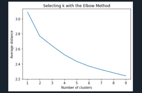
""" Plot average distance from observations from the cluster centroid to use the Elbow Method to identify number of clusters to choose """

plt.plot(clusters, meandist) plt.xlabel('Number of clusters') plt.ylabel('Average distance') plt.title('Selecting k with the Elbow Method')

Interpret 3 cluster solution model3=KMeans(n_clusters=3) model3.fit(clus_train) clusassign=model3.predict(clus_train)

plot clusters from sklearn.decomposition import PCA pca_2 = PCA(2) plot_columns = pca_2.fit_transform(clus_train) plt.scatter(x=plot_columns[:,0], y=plot_columns[:,1], c=model3.labels_,) plt.xlabel('Canonical variable 1') plt.ylabel('Canonical variable 2') plt.title('Scatterplot of Canonical Variables for 3 Clusters') plt.show()

""" BEGIN multiple steps to merge cluster assignment with clustering variables to examine cluster variable means by cluster """

create a unique identifier variable from the index for the cluster training data to merge with the cluster assignment variable clus_train.reset_index(level=0, inplace=True)

create a list that has the new index variable cluslist=list(clus_train['index'])

create a list of cluster assignments labels=list(model3.labels_)

combine index variable list with cluster assignment list into a dictionary newlist=dict(zip(cluslist, labels)) newlist

convert newlist dictionary to a dataframe newclus=DataFrame.from_dict(newlist, orient='index') newclus

rename the cluster assignment column newclus.columns = ['cluster']

now do the same for the cluster assignment variable create a unique identifier variable from the index for the cluster assignment dataframe to merge with cluster training data newclus.reset_index(level=0, inplace=True)

merge the cluster assignment dataframe with the cluster training variable dataframe by the index variable merged_train=pd.merge(clus_train, newclus, on='index') merged_train.head(n=100)

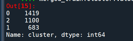
cluster frequencies merged_train.cluster.value_counts()

""" END multiple steps to merge cluster assignment with clustering variables to examine cluster variable means by cluster """

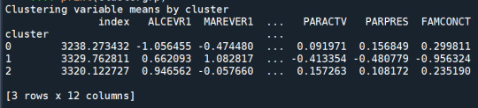
FINALLY calculate clustering variable means by cluster clustergrp = merged_train.groupby('cluster').mean() print ("Clustering variable means by cluster") print(clustergrp)

validate clusters in training data by examining cluster differences in GPA using ANOVA first have to merge GPA with clustering variables and cluster assignment data gpa_data=data_clean['GPA1']

split GPA data into train and test sets gpa_train, gpa_test = train_test_split(gpa_data, test_size=.3, random_state=123) gpa_train1=pd.DataFrame(gpa_train) gpa_train1.reset_index(level=0, inplace=True) merged_train_all=pd.merge(gpa_train1, merged_train, on='index') sub1 = merged_train_all[['GPA1', 'cluster']].dropna()

import statsmodels.formula.api as smf import statsmodels.stats.multicomp as multi

gpamod = smf.ols(formula='GPA1 ~ C(cluster)', data=sub1).fit() print (gpamod.summary())

print ('means for GPA by cluster') m1= sub1.groupby('cluster').mean() print (m1)

print ('standard deviations for GPA by cluster') m2= sub1.groupby('cluster').std() print (m2)

mc1 = multi.MultiComparison(sub1['GPA1'], sub1['cluster']) res1 = mc1.tukeyhsd() print(res1.summary())

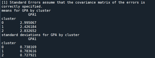
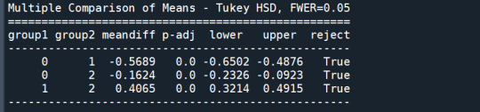
In order to externally validate the clusters, an Analysis of Variance (ANOVA) was conducting to test for significant differences between the clusters on grade point average (GPA). A tukey test was used for post hoc comparisons between the clusters. Results indicated significant differences between the clusters on GPA (F(3, 3197)=82.28, p<.0001). The tukey post hoc comparisons showed significant differences between clusters on GPA, with the exception that clusters 1 and 2 were not significantly different from each other. Adolescents in cluster 4 had the highest GPA (mean=2.99, sd=0.73), and cluster 3 had the lowest GPA (mean=2.42, sd=0.78).

[zhanariem]

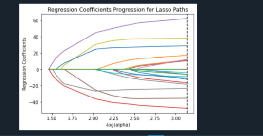
Week 3: Running a Lasso Regression Analysis

Warning ¡Change this line, deprecated code!

from sklearn.cross_validation import train_test_split

from sklearn.model_selection import train_test_split

Running in Linux Ubuntu

Installation in Linux Ubuntu.

sudo chmod +x Anaconda3-2022.10-Linux-x86_64.sh

./Anaconda3-2022.10-Linux-x86_64.sh

conda install scikit-learn

conda install -n my_environment scikit-learn

pip install sklearn

pip install -U scikit-learn scipy matplotlib

sudo apt-get install graphviz

sudo apt-get install pydotplus

conda create -c conda-forge -n spyder-env spyder numpy scipy pandas matplotlib sympy cython

conda create -c conda-forge -n spyder-env spyder

conda activate spyder-env

conda config --env --add channels conda-forge

conda config --env --set channel_priority strict

python -m pip install pydotplus

All predictor variables were standardized to have a mean of zero and a standard deviation of one.

Data were randomly split into a training set that included 70% of the observations (N=3201) and a test set that included 30% of the observations (N=1701). The least angle regression algorithm with k=10 fold cross validation was used to estimate the lasso regression model in the training set, and the model was validated using the test set. The change in the cross validation average (mean) squared error at each step was used to identify the best subset of predictor variables.

During the estimation process, self-esteem and depression were most strongly associated with school connectedness, followed by engaging in violent behavior and GPA. Depression and violent behavior were negatively associated with school connectedness and self-esteem and GPA were positively associated with school connectedness. Other predictors associated with greater school connectedness included older age, Hispanic and Asian ethnicity, family connectedness, and parental involvement in activities. Other predictors associated with lower school connectedness included being male, Black and Native American ethnicity, alcohol, marijuana, and cocaine use, availability of cigarettes at home, deviant behavior, and history of being expelled from school. These 18 variables accounted for 33.4% of the variance in the school connectedness response variable.

[zhanariem]

Week 2: Running a random forrest ¡Change this line, deprecated code!

from sklearn.cross_validation import train_test_split

from sklearn.model_selection import train_test_split

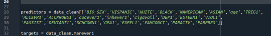
Random forest analysis was performed to evaluate the importance of series of explanatory variables in predicting a binary, categorical response variable. These are the following explanatory variables for evaluating smoking marijuana

The explanatory variables with the highest relative importance scores were ever smoked regulary (0.12081901) , drank alcohol (0.09069105) and deviant behavior scale (0.08861958).

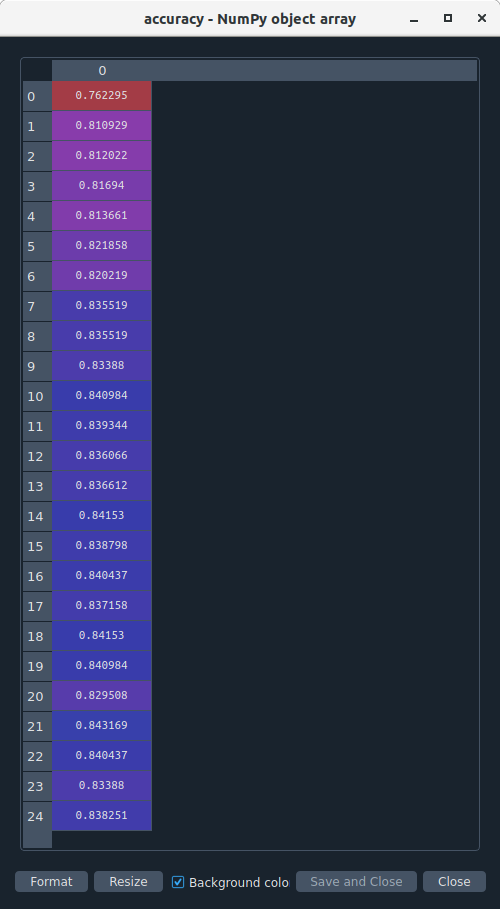
The accuracy of the random forest was 82%, with the subsequent growing of multiple trees rather than a single tree.

[zhanariem]

Week 1: Running Classification Tree (ubuntu linux)

Week 1 python decision trees As part of peer review assigment I am working on decision trees in Python. This assigment is intended for Coursera course “Machine Learning for Data Analysis by Wesleyan University”. 

Installation in Linux Ubuntu.

sudo chmod +x Anaconda3-2022.10-Linux-x86_64.sh

./Anaconda3-2022.10-Linux-x86_64.sh

conda install scikit-learn

conda install -n my_environment scikit-learn

pip install sklearn

pip install -U scikit-learn scipy matplotlib

sudo apt-get install graphviz

sudo apt-get install pydotplus

conda create -c conda-forge -n spyder-env spyder numpy scipy pandas matplotlib sympy cython

conda create -c conda-forge -n spyder-env spyder

conda activate spyder-env

conda config --env --add channels conda-forge

conda config --env --set channel_priority strict

python -m pip install pydotplus

dot -Tpng tree.dot -o tree5.png

I have to perform a decision tree analysis to test nonlinear relationships among a series of explanatory variables and a binary, categorical response variable. Data set is  provided by The National Longitudinal Study of Adolescent Health (AddHealth).

I will not complicate things here, therefore I am focusing on regular smoking (TREG1 variable).

I choosed few of vars to determine if they can predict regular smoking. predictor = dc[['HISPANIC','WHITE','BLACK','NAMERICAN','ASIAN']]

Therefore I did change predictor variables to just two: gender and age. I got this tree.

And my code?

!/usr/bin/env python3

-- coding: utf-8 --

""" Created on Wed Dec 28 11:06:15 2022

@author: rfernandez """ import numpy as np import pandas as pd import matplotlib.pylab as plt

from sklearn.cross_validation import train_test_split

from sklearn.model_selection import train_test_split from sklearn.tree import DecisionTreeClassifier from sklearn.metrics import classification_report from sklearn import tree import pydotplus import sklearn.metrics

#Load the dataset

data = pd.read_csv("tree_addhealth.csv")

dc = data.dropna() dc.dtypes dc.describe() """ Modeling and Prediction """

#Split into training and testing sets

predictor = dc[['HISPANIC','WHITE','BLACK','NAMERICAN','ASIAN']] target = dc.TREG1 pr_train,pr_test,t_train,t_test= train_test_split(predictor,target, test_size=0.4) pr_train.shape pr_test.shape t_train.shape t_test.shape

#Build model on training data

classif = DecisionTreeClassifier() classif = classif.fit(pr_train,t_train) pred=classif.predict(pr_test) sklearn.metrics.confusion_matrix(t_test,pred) sklearn.metrics.accuracy_score(t_test,pred)

#Displaying the decision tree

tree.export_graphviz(classif, out_file='tree_race.dot')

I translated .dot file to .png using “dot -Tpng name.dot -o name.png” command.