#categorization in dbms | Explore Tumblr posts and blogs

digitrenndsamr · 7 days ago

Text

RF Semiconductor Market to Record Sturdy Growth by 2031

Allied Market Research, titled, “RF Semiconductor Market," The RF semiconductor market was valued at $18.9 billion in 2021, and is estimated to reach $39.6 billion by 2031, growing at a CAGR of 8.4% from 2022 to 2031. The rapid development of 5G technology and the rapid adoption of IoT technology has increased the need for robust network capacity are some of the factors driving the RF Semiconductor market.

RF Power Semiconductors stands for Radio Frequency Power Semiconductors. These electronic devices are used for cellular and mobile wireless communications. There are numerous applications such as military radar, air and maritime traffic control systems. Various materials such as silicon, gallium arsenide, and silicon germanium are used to manufacture RF power semiconductors.

The growth of the RF semiconductor market is fueled by the massive adoption of AI technology. AI enhances business by improving the customer experience, enabling predictive maintenance and improving network reliability. By integrating effective machine learning algorithms, the company can reduce the design complexity of RF semiconductor devices and maximize RF parameters such as channel bandwidth, spectrum monitoring and antenna sensitivity. And while AI unlocks new capabilities for military applications, wireless applications in spectrum acquisition, communication systems, signal classification and detection in adverse spectrum conditions will also benefit greatly.

Robust network capacity has become essential with the proliferation of IoT technologies. IoT helps build a connected framework of physical things, such as smart devices, through secure networks using RF technology. For example, RF transceivers are used in smart home devices to connect to the internet via Bluetooth and Wi-Fi. Moreover, with the increasing number of smart city projects in various regions of the world, the demand for smart devices has increased significantly. In recent years, players in the RF semiconductor industry have been focused on product innovation, to stay ahead of their competitors. For instance: In January 2020, Qorvo Inc. launched the Qorvo QPG7015M IoT transceiver, which enables the simultaneous operation of all low-power, open-standard smart home technologies. Additionally, it is targeted at gateway IoT solutions that require the full-range capability of Bluetooth low energy (BLE), Zigbee, and Thread protocols, with +20 dBm (decibel per milliwatt) outputs.

The RF Semiconductor market is segmented on the basis of product type, application, and region. By product type, the market is segmented into RF power amplifiers, RF switches, RF filters, RF duplexers, and other RF devices. By application, the market is categorized into telecommunication, consumer electronics, automotive, aerospace & defense, healthcare, and others. Region-wise, the RF Semiconductor market is analyzed across North America (U.S., Canada, and Mexico), Europe (UK, Germany, France, and rest of Europe), Asia-Pacific (China, Japan, India, South Korea, and rest of Asia-Pacific) and LAMEA (Latin America, the Middle East, and Africa).

The outbreak of COVID-19 has significantly impacted the growth of the global RF Semiconductor sector in 2020, owing to the significant impact on prime players operating in the supply chain. On the contrary, the market was principally hit by several obstacles amid the COVID-19 pandemic, such as a lack of skilled workforce availability and delay or cancelation of projects due to partial or complete lockdowns, globally.

According to Minulata Nayak, Lead Analyst, Semiconductor and Electronics, at Allied Market Research, “The global RF Semiconductor market share is expected to witness considerable growth, owing to rising demand for the rapid development of 5G technology and the rapid adoption of IoT technology has increased the need for robust network capacity and has developed the RF semiconductor market size. On the other hand, the use of alternative materials such as gallium arsenide or gallium nitride improves device efficiency but also increases the cost of RF devices which is restraining the market growth during the anticipated period. Furthermore, the increased use of RF energy in the number of smart city projects in various countries around the world is creating opportunities for the RF Semiconductor market trends.”

According to RF Semiconductor market analysis, country-wise, the rest of the Asia-Pacific region holds a significant share of the global RF Semiconductor market, owing to the presence of prime players. Major organizations and government institutions in this country are intensely putting resources into these global automotive data cables. These prime sectors have strengthened the RF Semiconductor market growth in the region.

KEY FINDINGS OF THE STUDY

In 2021, by product type, the RF filters segment was the highest revenue contributor to the market, with $5,372.82 million in 2021, and is expected to follow the same trend during the forecast period.

By application, the consumer electronics segment was the highest revenue contributor to the market, with $6,436.63 million in 2021.

Asia-Pacific contributed the major share in the RF Semiconductor market, accounting for $7,937.05 million in 2021, and is estimated to reach $17,059.52 million by 2031, with a CAGR of 8.62%.

The RF Semiconductor market key players profiled in the report include Analog Devices Inc., Microchip Technology Inc., MACOM Technology, NXP Semiconductors, Qorvo, Inc., Qualcomm Incorporated, Texas Instruments Inc., Toshiba Electronic Devices & Storage Corporation, TDK Electronics, and Teledyne Technologies Inc. The market players have adopted various strategies, such as product launches, collaborations & partnerships, joint ventures, and acquisitions to expand their foothold in the RF Semiconductor industry.

#RF #Semiconductor #technology #electronics #artificial intelligence #ai generated #battery

1 note · View note

fromdevcom · 22 days ago

Text

A database management system (DBMS) is a software tool for efficiently carrying out database tasks such as insertion, retrieval, deletion, updating, organizing data into tables, views, schemas, and models. Based on how data is stored and handled, database systems are categorized into many different types. There are mainly four categories of database management systems.1. Hierarchical DatabasesData is organized in a tree-like hierarchical structure in hierarchical DBMSs, either in a bottom-up or top-down pattern. The hierarchy is linked through parent-child relationships in which a parent can have multiple children, but children can have just one parent.Hierarchical DBMSs commonly exhibit one-to-one and one-to-many types of relationships. As they have certain limitations, they are best suited only in very specific use cases. For example, each employee in a company reports to their respective departments. The department will act as a parent record, and each employee will represent child records. Each of them is linked back to that parent record in a hierarchical form. The IBM Information Management System (IMS) and Windows Registry are popular examples of hierarchical databases.2. Network DatabasesNetwork databases typically follow the network data model pattern. In this database type, data is represented in the form of nodes. Nodes connect with other neighboring nodes via links. In a network database, a node has the flexibility to share links with multiple nodes. This unique characteristic of sharing multiple links makes this database more efficient. A few popular examples are IDMS (Integrated Database Management System), Univac DMS-1100, Integrated Data Store (IDS), TurboIMAGE, and etc. 3. Relational DatabasesThe most commonly used database type today is a relational database. In a relational database (RDBMS), data is stored in tabular (rows and columns). Here, columns represent attributes, whereas rows represent a record or a tuple. Each field in a table represents a data value.One can use Structured Query Language (SQL) to query relational DBMSs with the help of operations like inserting, updating, deleting, and searching records.Usually, four types of relationships are seen in relational database design:one to one - In such a relationship 1 table record is related to another record in another table.one to many - In such a relationship 1 table record is related to multiple records in another table.many to one - In such a relationship more than 1 table record is related to another table record.many to many - In such a relationship multiple records are related to more than 1 record in another table.Some common examples of relational databases include MySQL, Microsoft SQL Server, Oracle, etc.4. Object-Oriented DatabasesThis type of database uses an object-based data model to save data. Data is stored in the form of objects. Each object contains two elements:A piece of data (e.g., sound, video, text, or graphics).Instructions or software commands are called methods to process the data.This type of database can easily integrate with object-oriented programming languages and utilize programming language capabilities. Object-oriented databases are compatible with many popular programming languages, including Delphi, JavaScript, Python, Java, C++, Perl, Scala, and Visual Basic. NET.We just discussed the four common database types. But wait! There are other popular databases that use different types of database structures. Examples like PostgreSQL (object-relational database) and NoSQL (non-tabular). Let's discuss these popular databases in some detail.PostgreSQLWhat is PostgreSQL? PostgreSQL or Postgres is an open-source object-relational database. PostgreSQL was first released on January 29, 1997, and, since then, its constant evolution has turned it into a reference for reliability, robustness, and performance. An object-relational database is a mix of object-based databases and relational databases to give you the best of both worlds.

It borrows object-oriented properties like table inheritance and function overloading which can help developers in handling complex database problems.PostgreSQL has rich driver support that allows popular technologies like Java, TypeScript, and Kotlin to connect and interact with the database.NoSQLNoSQL databases store data as JSON documents instead of tables (which are used in relational databases). NoSQL stands for ‘not only SQL’—it’s SQL and more. Very often, it is mistakenly understood as "no SQL". NoSQL offers the capability to save and query data without using SQL queries. That is how it get the name "noSQL". It offers the flexibility of JSON along with the power of SQL queries. NoSQL is gathering its popularity amongst modern businesses as it offers scalability and flexibility in its design. There are generally four types of NoSQL databases.Document databasesKey-value databasesWide-column databasesGraph databasesConclusionIn this write-up, we learned what a DBMS is and found out about some popular DBMSs out there. We also briefly read about the different categories of DBMSs based on their design. I hope you have a basic understanding of DBMSs. Thank you for being here with us. Join us to learn more about many different interesting topics.

0 notes

promptlyspeedyandroid · 1 month ago

Text

DBMS Tutorial Explained: Concepts, Types, and Applications

In today’s digital world, data is everywhere — from social media posts and financial records to healthcare systems and e-commerce websites. But have you ever wondered how all that data is stored, organized, and managed? That’s where DBMS — or Database Management System — comes into play.

Whether you’re a student, software developer, aspiring data analyst, or just someone curious about how information is handled behind the scenes, this DBMS tutorial is your one-stop guide. We’ll explore the fundamental concepts, various types of DBMS, and real-world applications to help you understand how modern databases function.

What is a DBMS?

A Database Management System (DBMS) is software that enables users to store, retrieve, manipulate, and manage data efficiently. Think of it as an interface between the user and the database. Rather than interacting directly with raw data, users and applications communicate with the database through the DBMS.

For example, when you check your bank account balance through an app, it’s the DBMS that processes your request, fetches the relevant data, and sends it back to your screen — all in milliseconds.

Why Learn DBMS?

Understanding DBMS is crucial because:

It’s foundational to software development: Every application that deals with data — from mobile apps to enterprise systems — relies on some form of database.

It improves data accuracy and security: DBMS helps in organizing data logically while controlling access and maintaining integrity.

It’s highly relevant for careers in tech: Knowledge of DBMS is essential for roles in backend development, data analysis, database administration, and more.

Core Concepts of DBMS

Let’s break down some of the fundamental concepts that every beginner should understand when starting with DBMS.

1. Database

A database is an organized collection of related data. Instead of storing information in random files, a database stores data in structured formats like tables, making retrieval efficient and logical.

2. Data Models

Data models define how data is logically structured. The most common models include:

Hierarchical Model

Network Model

Relational Model

Object-Oriented Model

Among these, the Relational Model (used in systems like MySQL, PostgreSQL, and Oracle) is the most popular today.

3. Schemas and Tables

A schema defines the structure of a database — like a blueprint. It includes definitions of tables, columns, data types, and relationships between tables.

4. SQL (Structured Query Language)

SQL is the standard language used to communicate with relational DBMS. It allows users to perform operations like:

SELECT: Retrieve data

INSERT: Add new data

UPDATE: Modify existing data

DELETE: Remove data

5. Normalization

Normalization is the process of organizing data to reduce redundancy and improve integrity. It involves dividing a database into two or more related tables and defining relationships between them.

6. Transactions

A transaction is a sequence of operations performed as a single logical unit. Transactions in DBMS follow ACID properties — Atomicity, Consistency, Isolation, and Durability — ensuring reliable data processing even during failures.

Types of DBMS

DBMS can be categorized into several types based on how data is stored and accessed:

1. Hierarchical DBMS

Organizes data in a tree-like structure.

Each parent can have multiple children, but each child has only one parent.

Example: IBM’s IMS.

2. Network DBMS

Data is represented as records connected through links.

More flexible than hierarchical model; a child can have multiple parents.

Example: Integrated Data Store (IDS).

3. Relational DBMS (RDBMS)

Data is stored in tables (relations) with rows and columns.

Uses SQL for data manipulation.

Most widely used type today.

Examples: MySQL, PostgreSQL, Oracle, SQL Server.

4. Object-Oriented DBMS (OODBMS)

Data is stored in the form of objects, similar to object-oriented programming.

Supports complex data types and relationships.

Example: db4o, ObjectDB.

5. NoSQL DBMS

Designed for handling unstructured or semi-structured data.

Ideal for big data applications.

Types include document, key-value, column-family, and graph databases.

Examples: MongoDB, Cassandra, Redis, Neo4j.

Applications of DBMS

DBMS is used across nearly every industry. Here are some common applications:

1. Banking and Finance

Customer information, transaction records, and loan histories are stored and accessed through DBMS.

Ensures accuracy and fast processing.

2. Healthcare

Manages patient records, billing, prescriptions, and lab reports.

Enhances data privacy and improves coordination among departments.

3. E-commerce

Handles product catalogs, user accounts, order histories, and payment information.

Ensures real-time data updates and personalization.

4. Education

Maintains student information, attendance, grades, and scheduling.

Helps in online learning platforms and academic administration.

5. Telecommunications

Manages user profiles, billing systems, and call records.

Supports large-scale data processing and service reliability.

Final Thoughts

In this DBMS tutorial, we’ve broken down what a Database Management System is, why it’s important, and how it works. Understanding DBMS concepts like relational models, SQL, and normalization gives you the foundation to build and manage efficient, scalable databases.

As data continues to grow in volume and importance, the demand for professionals who understand database systems is also rising. Whether you're learning DBMS for academic purposes, career development, or project needs, mastering these fundamentals is the first step toward becoming data-savvy in today’s digital world.

Stay tuned for more tutorials, including hands-on SQL queries, advanced DBMS topics, and database design best practices!

#dbms tutorial #what is dbms #How to learn dbms

0 notes

erpinformation · 9 months ago

Link

#DatabaseManagementSystem #DBMS

0 notes

digital-marketing-29 · 10 months ago

Text

What is SQL and Data Types ?

SQL (Structured Query Language) uses various data types to define the kind of data that can be stored in a database. Each SQL database management system (DBMS) may have its own variations, but here are the most common SQL data types categorized broadly:

Numeric Data Types INT (or INTEGER) Description: Used to store whole numbers. The typical range is -2,147,483,648 to 2,147,483,647. Example: sql CREATE TABLE Employees ( EmployeeID INT PRIMARY KEY, Age INT );

INSERT INTO Employees (EmployeeID, Age) VALUES (1, 30), (2, 25);

SELECT * FROM Employees WHERE Age > 28; DECIMAL (or NUMERIC) Description: Fixed-point numbers with a defined precision and scale (e.g., DECIMAL(10, 2) allows 10 digits total, with 2 after the decimal). Example: sql CREATE TABLE Products ( ProductID INT PRIMARY KEY, Price DECIMAL(10, 2) );

INSERT INTO Products (ProductID, Price) VALUES (1, 19.99), (2, 5.50);

SELECT * FROM Products WHERE Price < 10.00;

Character Data Types CHAR(n) Description: Fixed-length character string. If the input string is shorter than n, it will be padded with spaces. Example: sql CREATE TABLE Users ( UserID INT PRIMARY KEY, Username CHAR(10) );

INSERT INTO Users (UserID, Username) VALUES (1, 'Alice '), (2, 'Bob ');

SELECT * FROM Users; VARCHAR(n) Description: Variable-length character string that can store up to n characters. It does not pad with spaces. Example: sql CREATE TABLE Comments ( CommentID INT PRIMARY KEY, CommentText VARCHAR(255) );

INSERT INTO Comments (CommentID, CommentText) VALUES (1, 'Great product!'), (2, 'Not what I expected.');

SELECT * FROM Comments WHERE CommentText LIKE '%great%'; TEXT Description: Used for storing large amounts of text. The maximum length varies by DBMS. Example: sql CREATE TABLE Articles ( ArticleID INT PRIMARY KEY, Content TEXT );

INSERT INTO Articles (ArticleID, Content) VALUES (1, 'This is a long article content…');

SELECT * FROM Articles WHERE ArticleID = 1;

Date and Time Data Types DATE Description: Stores date values in the format YYYY-MM-DD. Example: sql CREATE TABLE Orders ( OrderID INT PRIMARY KEY, OrderDate DATE );

INSERT INTO Orders (OrderID, OrderDate) VALUES (1, '2024-01-15'), (2, '2024-02-10');

SELECT * FROM Orders WHERE OrderDate > '2024-01-01'; DATETIME Description: Combines date and time into one type, typically formatted as YYYY-MM-DD HH:MM:SS. Example: sql CREATE TABLE Appointments ( AppointmentID INT PRIMARY KEY, AppointmentTime DATETIME );

INSERT INTO Appointments (AppointmentID, AppointmentTime) VALUES (1, '2024-01-15 14:30:00');

SELECT * FROM Appointments WHERE AppointmentTime < NOW();

Binary Data Types BLOB (Binary Large Object) Description: Used to store large binary data, such as images or files. Example: sql Copy code CREATE TABLE Images ( ImageID INT PRIMARY KEY, ImageData BLOB );

-- Assume we have binary data for an image to insert -- INSERT INTO Images (ImageID, ImageData) VALUES (1, ?);

Boolean Data Type BOOLEAN Description: Stores TRUE or FALSE values. In some systems, this might be represented as TINYINT (0 for FALSE, 1 for TRUE). Example: sql CREATE TABLE Subscriptions ( SubscriptionID INT PRIMARY KEY, IsActive BOOLEAN );

INSERT INTO Subscriptions (SubscriptionID, IsActive) VALUES (1, TRUE), (2, FALSE);

SELECT * FROM Subscriptions WHERE IsActive = TRUE;

JSON and XML Data Types JSON Description: Stores JSON-formatted data, allowing for flexible data structures. Example: sql CREATE TABLE Users ( UserID INT PRIMARY KEY, UserInfo JSON );

INSERT INTO Users (UserID, UserInfo) VALUES (1, '{"name": "Alice", "age": 30}');

SELECT * FROM Users WHERE UserInfo->>'name' = 'Alice'; XML Description: Used for storing XML data, allowing for structured data storage. Example: sql CREATE TABLE Configurations ( ConfigID INT PRIMARY KEY, ConfigData XML );

INSERT INTO Configurations (ConfigID, ConfigData) VALUES (1, 'dark');

SELECT * FROM Configurations WHERE ConfigData.exist('/config/setting[@name="theme" and text()="dark"]') = 1;

Special Data Types ENUM Description: A string object with a value chosen from a list of permitted values. Example: sql CREATE TABLE Products ( ProductID INT PRIMARY KEY, Size ENUM('Small', 'Medium', 'Large') );

INSERT INTO Products (ProductID, Size) VALUES (1, 'Medium'), (2, 'Large');

SELECT * FROM Products WHERE Size = 'Medium'; SET Description: A string object that can have zero or more values, each of which must be chosen from a predefined list. Example: sql CREATE TABLE UserRoles ( UserID INT, Roles SET('Admin', 'Editor', 'Viewer') );

INSERT INTO UserRoles (UserID, Roles) VALUES (1, 'Admin,Editor'), (2, 'Viewer');

SELECT * FROM UserRoles WHERE FIND_IN_SET('Admin', Roles);

#what is sql

0 notes

toobler1 · 11 months ago

Text

Types of Application Software with Examples

Application software, often referred to simply as applications or apps, are programs designed to perform specific tasks for users. They are distinct from system software, which manages the fundamental operations of a computer. Application software can be categorized into several types based on their functionalities and uses. Here’s an overview of the different types of application software with relevant examples:

1. Word Processing Software

Description: This type of software is used for creating, editing, formatting, and printing text documents. It offers tools for text manipulation, spell checking, and various formatting options.

Examples: Microsoft Word, Google Docs, Apple Pages

2. Spreadsheet Software

Description: Spreadsheet software is used for organizing, analyzing, and storing data in tabular form. It provides functionalities for complex calculations, data analysis, and graphical representation of data.

Examples: Microsoft Excel, Google Sheets, Apple Numbers

3. Presentation Software

Description: Presentation software is used to create slideshows composed of text, images, videos, and other multimedia elements. These slideshows are typically used for educational, business, and professional presentations.

Examples: Microsoft PowerPoint, Google Slides, Apple Keynote

4. Database Management Software (DBMS)

Description: DBMS software is designed to create, manage, and manipulate databases. It allows users to store, retrieve, update, and delete data systematically.

Examples: MySQL, Microsoft SQL Server, Oracle Database

5. Graphic Design Software

Description: This software is used to create and manipulate visual content, such as images, illustrations, and graphics. It offers tools for photo editing, vector graphic creation, and digital painting.

Examples: Adobe Photoshop, CorelDRAW, GIMP

6. Web Browsers

Description: Web browsers are used to access and navigate the internet. They interpret and display web pages written in HTML, CSS, JavaScript, and other web technologies.

Examples: Google Chrome, Mozilla Firefox, Microsoft Edge, Safari

7. Email Clients

Description: Email client software is used to send, receive, and manage email messages. They offer functionalities like organizing emails, managing contacts, and integrating calendars.

Examples: Microsoft Outlook, Mozilla Thunderbird, Apple Mail

8. Multimedia Software

Description: Multimedia software is used to create, edit, and play audio and video files. It encompasses a range of tools for media playback, video editing, and sound recording.

Examples: VLC Media Player, Adobe Premiere Pro, Audacity

9. Accounting Software

Description: Accounting software is designed to manage financial transactions and records. It helps businesses track income, expenses, payroll, and other financial activities.

Examples: QuickBooks, FreshBooks, Xero

10. Project Management Software

Description: This software is used to plan, organize, and manage project tasks and resources. It aids in scheduling, tracking progress, and collaborating with team members.

Examples: Trello, Asana, Microsoft Project

To read more - 16 Types of Application Software with Examples

#application software

1 note · View note

uniathena · 1 year ago

Text

Level Up Your Data Game: Choosing the Perfect Online SQL Course with Certificate!

SQL is the dominant language for managing and manipulating data in this era of data revolution. In order to help you gain more valuable insights, make informed decisions, and progress your career, an SQL Online Course With Certificate can be your ideal starting point. Whether you want to take on matters related to Business by analyzing sales trends and optimizing the inventory level or Marketing, whereby understanding customer behaviour and campaign performance becomes the key, or aspire to join a group of Data Analysts, then learning SQL is a game changer.

What is SQL? SQL stands for Structured Query Language. It is a domain-specific language that is designed especially to manage relational databases. It is the language one uses when talking to the database, almost like using English to talk to another person. Using SQL, you can ask questions of your database (called queries) and get an answer in the form of data. The Power of SQL SQL is the backbone of modern data management an the key to unlocking the stored information in databases and getting valuable insights is SQL. SQL will allow you to aggregate, sort, filter, and query data to answer vital business inquiries define trends as well as drive data-informed decisions.

From big tech companies like Google and Amazon to individual startups or small business owners, no company can operate without SQL.It's a tool used by data analysts to find patterns, marketers to understand customers, financial analysts to track performance, and researchers to interpret results.These applications are endless hence making SQL a valuable asset for any career option. Why SQL Matters? It is a powerful tool that helps you to:

Get data: Frame specific questions to get the exact information required, like getting all customers who purchased in the last month or getting the list of best-selling products.

Insert data: Add new records, whether it is any new customer signing up with you or a new product added to your inventory.

Modify data: Modify existing records, e.g., a change to a customer's address, the price of some item, etc.

Remove data: Remove old or irrelevant records, keeping your database accurate and current.

SQL's Wide Reach SQL isn't limited to a single industry or profession. Business professionals across industries use it to solve a wide array of problems. Here are some examples:

Tech: Software Engineers use SQL to develop and maintain applications that work with databases. SQL is applied by data scientists during the extraction of data to be used in Machine Learning models. Database administrators use SQL to maintain and optimize database performance.

Finance: The reality is that financial analysts use SQL to track market trends, analyze investment portfolios, and create financial reports. Similarly, Risk Analysts utilize them to identify and manage risks in the same organization.

Marketing: Marketing professionals use SQL to categorize customers, personalize campaigns, and measure the effectiveness of marketing through website traffic data, among other means. This has led to its usage in analyzing website traffic and customer behavior. Healthcare: Healthcare analysts utilize SQL for activities such as analyzing patient data and identifying risk factors for specific diseases. They often use it for tracing disease outbreaks and establishing risk factors.

These are some examples of how SQL is used across industries. Its versatility makes it useful to anyone who deals with data.

UniAthena’s SQL: Beginner to Advanced Levels

With this SQL online course, you will learn the basics of database management concepts such as data types, DBMS, and RDBMS highlighting how SQL is used in efficient data administration. This is a self-paced online short course that prepares you to effectively utilize SQL, from simple queries to complex manipulations, within a 1-2 week period of learning that too for free. Plus, to top it all, upon successful completion of this course, earn yourself a Blockchain-verified SQL Certification to showcase your learning. Join now!

#online learning #online courses #short courses #free online courses #free online learning #free learning #free course #learn online #upskill online #free short courses #sql #sql course #sql certification

0 notes

innovativeroutinesinternational · 1 year ago

Text

The Comprehensive Guide to Data Migration Tools and Database Migration Tools

In today's fast-paced digital landscape, the need to move data efficiently and accurately from one environment to another is more critical than ever. Whether you're upgrading systems, consolidating data, or migrating to the cloud, data migration tools and database migration tools play a pivotal role in ensuring a smooth transition. This comprehensive guide will delve into what these tools are, their importance, the different types available, essential features to look for, and a review of some of the most popular tools on the market.

Understanding Data Migration Tools and Database Migration Tools

Data migration tools are software solutions designed to facilitate the process of transferring data between storage systems, formats, or computer systems. This can involve moving data between different databases, applications, or cloud environments. Database migration tools, a subset of data migration tools, specifically handle the transfer of database schemas and data between different database management systems (DBMS).

Importance of Data Migration Tools

Migrating data is a complex and risky task that can lead to data loss, corruption, or prolonged downtime if not executed correctly. Here are some reasons why data migration tools are essential:

1. Data Integrity: These tools ensure that data is accurately transferred without loss or corruption.

2. Efficiency: Automated tools speed up the migration process, reducing the time and resources required.

3. Minimal Downtime: Efficient data migration tools minimize downtime, ensuring business continuity.

4. Scalability: They can handle large volumes of data, making them suitable for enterprises of all sizes.

5. Compliance: Ensures adherence to regulatory requirements by maintaining data integrity and security during migration.

Types of Data Migration Tools

Data migration tools can be categorized based on their specific functions and the environments they operate in. Here are the main types:

1. On-Premises Tools: These tools are installed and operated within an organization's own infrastructure. They are suitable for migrating data between local systems or databases.

2. Cloud-Based Tools: These tools facilitate data migration to, from, or within cloud environments. They are ideal for organizations adopting cloud technologies.

3. Open-Source Tools: These are freely available tools that can be customized according to specific needs. They often have active community support but may require more technical expertise.

4. Commercial Tools: Paid solutions that come with professional support, advanced features, and comprehensive documentation. They are typically more user-friendly and scalable.

5. ETL Tools (Extract, Transform, Load): These tools are designed to extract data from one source, transform it into the desired format, and load it into the target system. They are commonly used in data warehousing and analytics projects.

Key Features to Look for in Data Migration Tools

When selecting data migration tools or database migration tools, consider the following essential features:

1. Ease of Use: User-friendly interfaces and intuitive workflows are crucial for reducing the learning curve and facilitating smooth migrations.

2. Data Mapping and Transformation: The ability to map and transform data from the source to the target schema is essential for ensuring compatibility and consistency.

3. Scalability: The tool should handle varying volumes of data and support complex migration scenarios.

4. Performance: High-performance tools reduce migration time and minimize system downtime.

5. Error Handling and Reporting: Robust error handling, logging, and reporting features help identify and resolve issues quickly.

6. Security: Ensuring data security during migration is critical. Look for tools with encryption and compliance features.

7. Support and Documentation: Comprehensive support and detailed documentation are vital for troubleshooting and effective tool utilization.

Popular Data Migration Tools

Here are some of the most popular data migration tools and database migration tools available:

1. AWS Database Migration Service (DMS): AWS DMS is a cloud-based service that supports database migrations to and from Amazon Web Services. It is highly scalable, supports homogeneous and heterogeneous migrations, and provides continuous data replication.

2. Azure Database Migration Service: This tool from Microsoft facilitates the migration of databases to Azure. It supports various database management systems, offers automated assessments, and provides seamless integration with other Azure services.

3. Talend: Talend is an ETL tool that offers robust data integration and migration capabilities. It supports numerous data sources and formats, providing a visual interface for designing data workflows and transformations.

4. IBM InfoSphere DataStage: IBM InfoSphere DataStage is a powerful ETL tool designed for large-scale data integration projects. It offers advanced data transformation capabilities, high performance, and extensive support for various data sources.

5. Oracle Data Integrator (ODI): ODI is a comprehensive data integration platform from Oracle that supports ETL and ELT architectures. It provides high-performance data transformation and integration capabilities, making it suitable for complex migration projects.

6. Fivetran: Fivetran is a cloud-based data integration tool that automates data extraction, transformation, and loading. It supports numerous data sources and destinations, providing seamless data synchronization and real-time updates.

7. Apache Nifi: Apache Nifi is an open-source data integration tool that supports data migration, transformation, and real-time data processing. It offers a web-based interface for designing data flows and extensive customization options.

8. Hevo Data: Hevo Data is a cloud-based data integration platform that offers real-time data migration and transformation capabilities. It supports various data sources, provides automated data pipelines, and ensures high data accuracy.

Best Practices for Using Data Migration Tools

To ensure successful data migrations, follow these best practices:

1. Plan Thoroughly: Define your migration strategy, scope, and timeline. Identify potential risks and develop contingency plans.

2. Data Assessment: Evaluate the quality and structure of your source data. Cleanse and normalize data to ensure compatibility with the target system.

3. Pilot Testing: Conduct pilot migrations to test the tools and processes. This helps identify and resolve issues before full-scale migration.

4. Monitor and Validate: Continuously monitor the migration process and validate the data at each stage. Ensure that data integrity and consistency are maintained.

5. Minimize Downtime: Schedule migrations during low-traffic periods and implement strategies to minimize downtime, such as phased migrations or parallel processing.

6. Documentation and Training: Document the migration process and provide training to the team members involved. This ensures a smooth transition and helps address any post-migration issues.

Conclusion

Data migration tools and database migration tools are indispensable for modern businesses looking to upgrade systems, consolidate data, or migrate to the cloud. These tools offer automated, efficient, and secure methods for transferring data, ensuring data integrity and minimizing downtime. With a variety of tools available, ranging from open-source solutions to commercial platforms, businesses can choose the one that best fits their needs and requirements. By following best practices and leveraging the right tools, organizations can achieve successful data migrations, paving the way for improved operations and business growth.

As you embark on your data migration journey, remember to carefully evaluate your options, plan meticulously, and prioritize data security and integrity. With the right approach and tools, you can ensure a seamless and successful data migration process.

#database migration tools #data migration tools

0 notes

mulemasters · 1 year ago

Text

Cardinality in DBMS Tosca

Understanding Cardinality in DBMS: A Guide for Tosca Users

In the world of Database Management Systems (DBMS), understanding the concept of cardinality is crucial for designing efficient and effective databases. Cardinality, in essence, refers to the uniqueness of data values contained in a column. When dealing with DBMS and testing automation tools like Tosca, a solid grasp of cardinality can significantly improve your database interactions and testing accuracy.

What is Cardinality?

Cardinality in DBMS describes the relationships between tables and the uniqueness of data values. It plays a pivotal role in database design and helps in defining the relationships between tables in a relational database. Cardinality is typically categorized into three types:

One-to-One (1:1): Each record in one table corresponds to one and only one record in another table. For example, in a school database, each student might have a unique student ID, linking them to a single record in the student details table.

One-to-Many (1:N): A single record in one table can be associated with multiple records in another table. For instance, a single teacher can teach multiple students. Therefore, the teacher's table will have a one-to-many relationship with the student's table.

Many-to-Many (N:M): Records in one table can be associated with multiple records in another table and vice versa. For example, students can enroll in multiple courses, and each course can have multiple students enrolled. This type of relationship is often managed through a junction table.

Importance of Cardinality in DBMS

Understanding cardinality is vital for several reasons:

Database Design: Properly defining relationships between tables ensures data integrity and efficient query performance. Misinterpreting cardinality can lead to redundant or inconsistent data.

Query Optimization: Knowing the cardinality helps in writing optimized SQL queries. For example, when joining tables, understanding the relationship between them can help you avoid unnecessary data duplication.

Data Integrity: Cardinality constraints ensure that the relationships between tables are maintained, preventing orphaned records and ensuring that data is consistently related across the database.

Cardinality and Tosca

Tosca, a popular test automation tool, relies heavily on database interactions for data-driven testing and validation. Understanding cardinality can enhance your ability to create robust and accurate tests in Tosca. Here's how:

Test Data Management: By understanding the relationships between different tables, you can ensure that your test data accurately reflects real-world scenarios. This leads to more reliable and meaningful test results.

Test Case Design: Knowledge of cardinality helps in designing test cases that cover all possible data relationships. For example, when testing a student enrollment system, you would need to consider one-to-many relationships to validate that each student can enroll in multiple courses correctly.

Efficient Query Writing: When creating automated tests that involve database queries, knowing the cardinality can help you write efficient and effective SQL statements, ensuring that your tests run smoothly and quickly.

Validation of Data Integrity: Automated tests in Tosca can include checks for data integrity based on cardinality rules. This ensures that the database maintains correct relationships and prevents issues like duplicate entries or orphaned records.

Conclusion

In the realm of DBMS and test automation with Tosca, understanding cardinality is more than just a theoretical concept—it's a practical necessity. It enhances your ability to design efficient databases, write optimized queries, and create robust automated tests. By mastering cardinality, you can ensure data integrity, improve performance, and deliver more reliable software solutions.

Ready to take your Tosca skills to the next level? Dive deep into the world of DBMS with a focus on cardinality, and unlock the full potential of your database testing and automation capabilities.

#tosca pipeline #tosca development #tosca client #tosca with jenkins #tosca course #tosca Training #cardinality dbms

1 note · View note

enterprisewired · 1 year ago

Text

Structured vs. Unstructured Data: What’s The Difference?

Businesses and organizations generate and analyze vast amounts of information. This information can be broadly classified into two categories: structured vs. unstructured data. Understanding the differences between these types of data and their respective applications is crucial for effective data management and analysis. This article explores the characteristics, benefits, challenges, and use cases of structured and unstructured data.

What is Structured Data?

Structured data is organized and formatted in a way that makes it easily searchable and analyzable by computers. This type of data is typically stored in databases and spreadsheets, where it can be systematically arranged in rows and columns. Examples of structured data include:

Relational Databases: Customer information, transaction records, and product inventories.

Spreadsheets: Financial data, sales figures, and employee details.

Characteristics of Structured Data

Organized Format: Structured data is highly organized, usually in tables with defined columns and rows.

Easily Searchable: Due to its organization, structured data can be easily queried and retrieved using database management systems (DBMS).

Fixed Schema: Structured data follows a predetermined schema, meaning the data types and relationships are defined in advance.

Quantitative: Structured data is often numerical or categorical, allowing for straightforward statistical analysis.

Benefits of Structured Data

Ease of Analysis: Structured data can be easily analyzed using SQL queries, data mining tools, and business intelligence software.

Efficiency: The organized nature of structured data allows for efficient storage, retrieval, and management.

Accuracy: Structured data tends to have high accuracy and consistency due to its adherence to a defined schema.

Challenges of Structured Data

Rigidity: The fixed schema of structured data makes it less flexible when dealing with changes or additions to the data structure.

Limited Scope: Structured data is often limited to numerical and categorical information, excluding more complex data types like text, images, and videos.

What is Unstructured Data?

Unstructured data lacks a predefined format or organization, making it more complex to process and analyze. This type of data is generated in a variety of formats, including text, images, videos, and audio files. Examples of unstructured data include:

Text Documents: Emails, social media posts, and web pages.

Multimedia: Images, videos, and audio recordings.

Sensor Data: Data from IoT devices, such as temperature readings and GPS coordinates.

Characteristics of Unstructured Data

Lack of Structure: Unstructured data does not follow a specific format or organization.

Diverse Formats: It can exist in various formats, including text, images, audio, and video.

Qualitative: Unstructured data is often qualitative, containing rich information that requires advanced techniques to analyze.

Benefits of Unstructured Data

Rich Information: Unstructured data provides a wealth of information that can offer deep insights into behaviors, trends, and patterns.

Flexibility: It can capture complex and diverse data types, making it suitable for a wide range of applications.

Real-World Relevance: Much of the data generated in the real world is unstructured, making it highly relevant for many use cases.

Challenges of Unstructured Data

Complexity: Analyzing unstructured data requires advanced techniques such as natural language processing (NLP), image recognition, and machine learning.

Storage and Management: Unstructured data requires more storage space and sophisticated management systems compared to structured data.

Searchability: Retrieving specific information from unstructured data can be challenging without proper indexing and search algorithms.

Applications of Structured and Unstructured Data

Structured Data Applications

Business Intelligence: Structured data is the backbone of business intelligence systems, providing actionable insights through data analytics and reporting.

Financial Analysis: Financial institutions use structured data for analyzing transactions, risk assessment, and regulatory compliance.

Customer Relationship Management (CRM): Structured data helps businesses manage customer information, track interactions, and improve customer service.

Unstructured Data Applications

Sentiment Analysis: Companies analyze social media posts, reviews, and other text data to understand customer sentiment and improve products or services.

Multimedia Content Analysis: Unstructured data from images and videos is used in facial recognition, video surveillance, and content recommendation systems.

IoT and Sensor Data: Unstructured data from IoT devices is used for predictive maintenance, smart city applications, and environmental monitoring.

Integrating Structured vs. Unstructured Data

To fully leverage the power of both structured and unstructured data, businesses are increasingly adopting hybrid approaches that combine these data types. Techniques such as data warehousing, data lakes, and big data platforms enable the integration and analysis of diverse data sources. Here are some ways to achieve this integration:

Data Lakes: Data lakes store structured and unstructured data in its raw form, allowing for flexible analysis and processing using big data technologies.

Data Warehousing: Traditional data warehouses can be extended to incorporate unstructured data by using data transformation and integration tools.

Big Data Analytics: Platforms like Hadoop and Spark provide the infrastructure to process and analyze large volumes of structured and unstructured data.

Conclusion

Understanding the differences between structured vs. unstructured data is crucial for effective data management and analysis. While structured data offers ease of analysis and efficiency, unstructured data provides rich, qualitative insights that can drive innovation and competitive advantage.

By integrating and leveraging both types of data, businesses can unlock new opportunities, enhance decision-making, and achieve a comprehensive view of their operations and market dynamics. As technology continues to evolve, the ability to manage and analyze structured and unstructured data will become increasingly important for organizations aiming to thrive in the data-driven era.

0 notes

digitrenndsamr · 10 months ago

Text

RF Semiconductor Market to Receive Overwhelming Hike in Revenues By 2031

KEY FINDINGS OF THE STUDY

By application, the consumer electronics segment was the highest revenue contributor to the market, with $6,436.63 million in 2021.

Asia-Pacific contributed the major share in the RF Semiconductor market, accounting for $7,937.05 million in 2021, and is estimated to reach $17,059.52 million by 2031, with a CAGR of 8.62%.

0 notes

sanaablog1 · 1 year ago

Text

Assignment 3

Lasso regression analysis for shrinkage variable selection in the banking system

Introduction:

A personal equity plan (PEP) was an investment plan introduced in the United Kingdom that encouraged people over the age of 18 to invest in British companies. Participants could invest in shares, authorized unit trusts, or investment trusts and receive both income and capital gains free of tax. The PEP was designed to encourage investment by individuals. Banks engage in data analysis related to Personal Equity Plans (PEPs) for various reasons. They use it to assess the risk associated with these investment plans. By examining historical performance, market trends, and individual investor behavior, banks can make informed decisions about offering PEPs to their clients.

In general, banks analyze PEP-related data to make informed investment decisions, comply with regulations, and tailor their offerings to customer needs. The goal is to provide equitable opportunities for investors while managing risks effectively.

SAS Code

LIBNAME mylib "/home/u63879373";

proc import out=mylib.mydata datafile='/home/u63879373/bank.csv' dbms=CSV replace;

proc print data=mylib.mydata;

run;

/*********DATA MANAGEMENT****************/

data new; set mylib.mydata; /*using numerical values for new variables*/

if pep="YES" then res=1; else res=0;

if sex="MALE" then gender=1; else gender=0;

if married="YES" then status=1; else status=0;

if car="YES" then cars=1; else cars=0;

if save_act="YES" then save=1; else save=0;

if current_act="YES" then current=1; else current=0;

if mortgage="YES" then mortg=1; else mortg=0;

ods graphics on;

* Split data randomly into test and training data;

proc surveyselect data=new out=traintest seed = 123 samprate=0.7 method=srs outall;

Run;

* lasso multiple regression with lars algorithm k=10 fold validation;

proc glmselect data=traintest plots=all seed=123;

partition ROLE=selected(train='1' test='0');

model res=age gender income status children cars save

current mortg/selection=lar(choose=cv stop=none) cvmethod=random(10);

RUN;

Dataset

The dataset I used in this assignment contains information about customers in a bank. The Data analysis used will help the bank take know the important features that can affect the PEP of a client from the following features: age, sex, region, income, married, children, car, save_act, current_act and the mortgage.

Id: a unique identification number,

age: age of customer in years (numeric),

income: income of customer (numeric)

sex: MALE / FEMALE

married: is the customer married (YES/NO)

children: number of children (numeric)

car: does the customer own a car (YES/NO)

save_acct: does the customer have a saving account (YES/NO)

current_acct: does the customer have a current account (YES/NO)

mortgage: does the customer have a mortgage (YES/NO)

Figure1: dataset

Lasso Regression

LASSO is a shrinkage and variable selection method for linear regression models. The goal of lasso regression is to obtain the subset of predictors that minimizes prediction error for a quantitative response variable. The lasso does this by imposing a constraint on the model parameters that causes regression coefficients for some variables to shrink toward zero. Variables with a regression coefficient equal to zero after the shrinkage process are excluded from the model. Variables with non-zero regression coefficients variables are most strongly associated with the response variable. Explanatory variables can be either quantitative, categorical or both.

In this assignement, we will use Lasso on the above dataset to identify a set of variables that best predicts the binary response variable which is the pep for the bank customers.

Lasso Regression Analysis

I used the libname statement to call my dataset.

data management: I created new variables that will hold numerical values instead of the string values we had in the table:

for the pep variable res=1; if pep is yes and res=0 otherwise;

if sex="MALE" then gender=1; else gender=0; 0 for Female and 1 for Male

if married="YES" then status=1; else status=0; the customer is married or not

if car="YES" then cars=1; else cars=0; the customer has a car or not

if save_act="YES" then save=1; else save=0; the customet has a saving account or not

if current_act="YES" then current=1; else current=0; the customer has a current account or not

if mortgage="YES" then mortg=1; else mortg=0; the customer has a mortgage or not

The SURVEYSELECT procedure

ODS graphics is turned on for the SAS to plot graphics. The data set is randomly split into a training data set consisting of 70% of the total observations in the data set, and a test data set consisting of the other 30% of the observations as seen in the figure below.

Figure 2

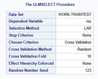
The GLMSELECT procedure

This figure shows information about the Lasso regression. The dependent Variable, res (which is the pep in the bank table), and the LAR selection method used. It also shows that I used as a criterion for choosing the best model, K equals 10-fold cross validation, with random assignments of observations to the folds.

Figure 3

The GLMSELECT procedure

The figure below shows the total number of observations in the data set, 600 observations, which is the same as the number of observations used for training and testing the statistical models.

It shows also the number of parameters to be estimated which is 10 for the intercept plus the 9 predictors.

Figure 4

The LAR Selection summary

The next figure shows information about the LAR selection. It shows the steps in the analysis and the variable that is entered at each step. We can see that the variables are entered as follows, income then status (married or not), then age, and so on.

Figure 5

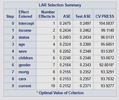
At the beginning, there are no predictors in the model. Just the intercept. Then variables are entered one at a time in order of the magnitude of the reduction in the mean, or average squared error (ASE). The variables are ordered in terms of how important they are in predicting the customer’s PEP. From the figure and according to the lasso regression results, we can see that the most important predictor of the PEP is the customer’s income, then whether the customer is married or not then the age and so on. You can also see how the average square error declines as variables are added to the model, indicating that the prediction accuracy improves as each variable is added to the model.

The CV PRESS shows the sum of the residual sum of squares in the test data set. There's an asterisk at step 6. This is the model selected as the best model by the procedure since it is the model with the lowest summed residual sum of squares and that adding other variables to this model, actually increases it.

Finally, we can see that the training data ASE continues to decline as variables are added. This is to be expected as model complexity increases.

Coefficient Progression

Next figure shows the change in the regression coefficients at each step, and the vertical line represents the selected model. The plot shows the relative importance of the predictor selected at any step of the selection process, how the regression coefficients changed with the addition of a new predictor at each step as well as the steps at which each variable entered the model. For example, as also indicated in the summary table above, the customer’s income has the largest regression coefficient, followed by married then the age.

We can also see that the number of children and whether the customer has a mortgage or not are negatively associated with the PEP.

The lower plot shows how the chosen selection criterion, in this example CVPRESS, which is the residual sum of squares summed across all the cross-validation folds in the training set, changes as variables are added to the model.

Initially, it decreases rapidly and then levels off to a point in which adding more predictors doesn't lead to much production in the residual sum of squares.

Figure 6

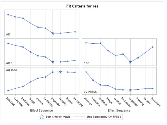
Fit criteria for pep

The figure plot shows at which step in the selection process different selection criteria would choose the best model. Interestingly, the other, criteria selected more complex models, and the criterion based on cross validation, possibly selecting an overfitted model.

Figure 7

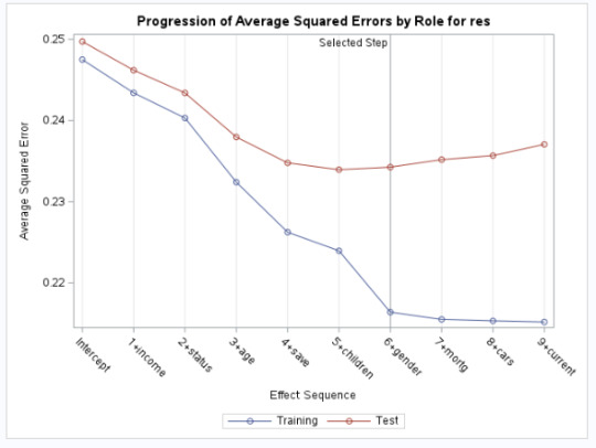
Progression of average square errors by Role for the PEP (res)

The next figure shows the change in the average or mean square error at each step in the process. As expected, the selected model was less accurate in predicting the PEP in the test data, but the test average squared error at each step was pretty close to the training average squared error especially for the first important variables.

Figure 8

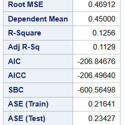
Analysis of variance

The figure below shows the R-Square (0.1256) and adjusted R-Square (0.1129) for the selected model and the mean square error for both the training (0.21)and test data (0.23).

Figure 9

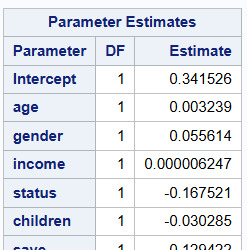
Parameter estimates

The goal of lasso regression is to obtain the subset of predictors that minimizes prediction error for a quantitative response variable. Variables with a regression coefficient equal to zero after the shrinkage process are excluded from the model. So, we can see from the results that the two variables current_act and car variables were excluded as they are not associated with the PEP response variable. The other variables age, sex(gender), and income variables are most strongly associated with the response variable.

Conclusion

Lasso regression is a supervised machine learning method often used in machine learning to select the subset of variables. It is a Shrinkage and Variable Selection method for linear regression models. Lasso Regression is useful because shrinking the regression coefficient can reduce variance without a substantial increase in bias. However, without human intervention, variable selection methods could produce models that make little sense or that turn out to be useless for accurately predicting a response variable in the real world. If machine learning, human intervention, and independent application are combined, we will get better results and therefore better predictions.

0 notes

mengchunhsieh · 1 year ago

Text

Assignment 2:

Finding important features to predict the personal equity plan (PEP) in the banking system

Introduction:

SAS Code

proc import out=mydata

datafile="/home/u63879373/bank.csv"

dbms=csv

replace;

getnames=YES;

PROC SORT; BY id;

ods graphics on;

PROC HPFOREST;

target PEP/level=nominal; /*target variable*/

input sex region married children car save_act current_act mortgage /level=nominal;

input age income /level=interval ;

RUN;

Dataset

Id: a unique identification number,

age: age of customer in years (numeric),

income: income of customer (numeric)

sex: MALE / FEMALE

married: is the customer married (YES/NO)

region: inner_city/rural/suburban/town

children: number of children (numeric)

car: does the customer own a car (YES/NO)

save_acct: does the customer have a saving account (YES/NO)

current_acct: does the customer have a current account (YES/NO)

mortgage: does the customer have a mortgage (YES/NO)

Figure1: dataset

Random Forest

Random forests are predictive models that allow for a data driven exploration of many explanatory variables in predicting a response or target variable. Random forests provide important scores for each explanatory variable and also allow you to evaluate any increases in correct classification with the growing of smaller and larger number of trees.

Random forest was used on the above dataset to evaluate the importance of a series of explanatory variables in predicting a binary, categorical response variable (PEP).

Following the import to import the dataset, I will include PROC HPFOREST. Next, I name my response, or target variable, PEP which is a nominal variable.

For the input statements I indicate the following:

Sex, region, married, children, car, save_act, current_act, and mortgage are nominal variables (categorical explanatory variables).

Age and income are interval variables (Quantitative explanatory variables).

Random Forest Analysis:

After running the code above we get the following results:

Model information

Figure2: Model of Information

We can see from the model that variables to try is equal to 3, indicating that a random selection of three explanatory variables was selected to test each possible split for each node in each tree within the forest.

SAS will grow 100 trees by default and select 60% of their sample when performing the bagging process (inbag fraction=0.6).

The prune fraction is equal to the default value: 0 which means that the tree is not to prune.

Leaf size specifies the smallest number of training observations that a new branch can have. The default value is 1.

The split criteria used in HPFOREST is the Gini index.

Missing value: Valid value since the target variable is not missing.

Number of Observations

Figure 3

The number of observations read from my data set is the same as the number of observations used (N= 600 for both number of observations).

For the baseline fit statistics output, the misclassification rate of the RF is 0.457. So, the algorithm misclassified 45.7% of the sample and the remaining 54.3% of the data were correctly classified (1-0.457=0.543).

Fit Statistics for 1 to 100 number of trees

PROC HPFOREST computes fit statistics for a sequence of forests that have an increasing number of trees. As the number of trees increases, the fit statistics usually improve. And this can be seen by the decreasing value of the average square error as the number of trees increases.

for 1 tree ASE (train)=0.1354, ASE (OOB)=0.211

for 10 trees ASE (train)=0.0810, ASE (OOB)=0.178

Figure 4: 10 first forests

for 90 trees ASE (train)=0.0716, ASE (OOB)=0.147

for 100 trees ASE (train)=0.0712, ASE (OOB)=0.146

Figure 5: 10 last forests

For the out of bag misclassification rate (OOB), we can notice that we get a near perfect prediction in the training samples as the number of trees grown gets closer to 100. When those same models are tested on the out of bag sample, the misclassification rate is around 17% (0.172 for 100 number of trees). OOB estimate is a convenient substitute for an estimate that is based on test data and is a less biased estimate of how the model will perform on future data.

Variable Importance Ranking

Figure 6: Loss Reduction Variable Importance

The final table in the output table for the random forest algorithms applied to this dataset which is the variable importance rankings. The number of rules column shows the number of splitting rules that use a variable. Each measure is computed twice, once on training data and once on the out of bag data. As with fit statistics, the out of bag estimates are less biased. The rows are sorted by the OOB Gini measure.

The variables are listed from highest importance to lowest importance in predicting the PEP value. Here we see that some of the most important variables in predicting the PEP for a client is the number of children, then whether he is married or not, whether he has a mortgage or not, whether he has a saving then current accounts, whether he has a car or not, his sex, his region, the income and age come at the end which means those are the least important values to decide determine his PEP value.

Conclusion

Random forests are a type of data mining algorithm that can select from among a large number of variables, those that are most important in determining the target or response variable to be explained. The target and the explanatory variables can be categorical or quantitative, or any combination. The forest of trees is used to rank the importance of variables in predicting the target. In this way, random forests are sometimes used as a data reduction technique, where variables are chosen in terms of their importance to be included in regression and other types of future statistical models.

爆發

0 則迴響

0 notes

sidslash918 · 1 year ago

Text

Data Analysis Tools - Week 1 Assignment

Gapminder dataset variables:

incomeperperson 2010 Gross Domestic Product per capita in constant 2000 US$. The inflation but not the differences in the cost of living

polityscore 2009 Democracy score (Polity) Overall polity score from the Polity IV dataset, calculated by subtracting an autocracy score from a democracy score. The summary measure of a country's democratic and free nature. -10 is the lowest value, 10 the highest.

urbanrate 2008 urban population (% of total) Urban population refers to people living in urban areas as defined by national statistical offices (calculated using World Bank population estimates and urban ratios from the United Nations World Urbanization Prospects).

Syntax of the code used:

Libname data '/home/u47394085/Data Analysis and Interpretation';

Proc Import Datafile='/home/u47394085/Data Analysis and Interpretation/gapminder.csv' Out=data.Gapminder Dbms=csv replace; Run;

Data Gapminder; Set data.Gapminder; Format IncomeGroup $30. PoliticalStability $20. Urbanization $10.; If incomeperperson=. Then IncomeGroup='NA'; Else If incomeperperson>0 and incomeperperson<=1500 Then IncomeGroup='Lower'; Else If incomeperperson>1500 and incomeperperson<=4500 Then IncomeGroup='Lower Middle'; Else If incomeperperson>4500 and incomeperperson<=15000 Then IncomeGroup='Upper Middle'; Else IncomeGroup='Upper';

If polityscore=. Then PoliticalStability='NA'; Else If polityscore<5 Then PoliticalStability='Unstable'; Else PoliticalStability='Stable';

If urbanrate=. Then Urbanization='NA'; Else If urbanrate<50 Then Urbanization='Low'; Else Urbanization='High'; Run;

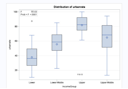
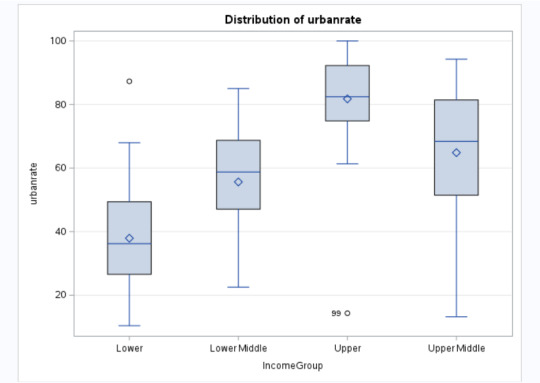
Proc Anova Data=Gapminder; Class IncomeGroup; Model urbanrate=IncomeGroup; Means IncomeGroup / Duncan; Where IncomeGroup NE 'NA'; Run;

Since the Gapminder dataset provided has quantitative variables, the variables incomeperperson, polityscore and urbanrate have been turned into categorical variables IncomeGroup, PoliticalStability and Urbanization respectively.

Anova Test

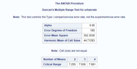
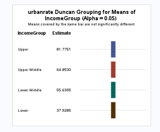
Proc Anova Data=Gapminder; Class IncomeGroup; Model urbanrate=IncomeGroup; Means IncomeGroup / Duncan; Where IncomeGroup NE 'NA'; Run;

Through ANOVA we want to explore the statistical significance of the categorical variable IncomeGroup on the quantitative response variable urbanrate. The Post Hoc Test Comparison used was DUNCAN.

Null Hypothesis: There is no relationship between Income levels and urbanization in a country.

Alternate Hypothesis: There is a relationship between Income levels and urbanization in a country.

Results Screenshots

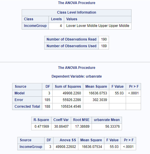
Explanation:

Since the p <0.05, we can reject the null hypothesis and say that there is a relationship between IncomeGroup and Urbanrate. Further studying, we see that higher the income, higher is the urbanization. The IncomeGroups Lower, Lower Middle, Upper Middle and Upper are statistically different when compared against Urbanization.

0 notes

edcater · 1 year ago

Text

Learn SQL Programming from the Ground Up: Beginner-Friendly Tutorial

Are you ready to dive into the world of databases and take your first steps in SQL programming? Whether you're a budding data scientist, a web developer, or simply curious about managing data effectively, learning SQL (Structured Query Language) is a valuable skill that can open up a plethora of opportunities. In this beginner-friendly tutorial, we'll guide you through the fundamentals of SQL in a simple and easy-to-understand manner.

Understanding Databases and SQL

Before we delve into SQL, let's understand what databases are and why SQL is essential. Imagine a database as a structured collection of data organized for efficient retrieval, manipulation, and storage. SQL acts as the language used to interact with these databases, enabling users to perform various operations such as querying, updating, and managing data.

Setting Up Your Environment

To start your SQL journey, you'll need access to a database management system (DBMS) such as MySQL, PostgreSQL, or SQLite. These systems provide a platform to create and interact with databases using SQL commands. You can choose to install one locally on your computer or use online platforms offering SQL sandboxes for practice.

Getting Started with SQL Syntax

SQL commands are categorized into different types, including Data Definition Language (DDL), Data Manipulation Language (DML), Data Query Language (DQL), and Data Control Language (DCL). Let's explore some basic SQL syntax:

Creating a Database:

sql

Copy code

CREATE DATABASE database_name;

Creating a Table:

sql

Copy code

CREATE TABLE table_name (

column1 datatype,

column2 datatype,

...

);

Inserting Data:

sql

Copy code

INSERT INTO table_name (column1, column2, ...)

VALUES (value1, value2, ...);

Querying Data:

sql

Copy code

SELECT column1, column2, ...

FROM table_name

WHERE condition;

Understanding Data Types

In SQL, each column in a table has a specific data type that defines the kind of data it can store. Common data types include INTEGER, VARCHAR, DATE, and BOOLEAN. It's crucial to choose appropriate data types based on the nature of the data you're working with to ensure accuracy and efficiency in your database operations.

Retrieving Data with SELECT Statements

The SELECT statement is one of the most fundamental SQL commands used for retrieving data from a database. Let's break down its syntax:

sql

Copy code

SELECT column1, column2, ...

FROM table_name

WHERE condition;

You can select specific columns or retrieve all columns using an asterisk (*) wildcard. The WHERE clause allows you to specify conditions for filtering data based on certain criteria.

Modifying Data with UPDATE and DELETE Statements

In addition to querying data, SQL allows you to modify existing records in a database using the UPDATE statement:

sql

Copy code

UPDATE table_name

SET column1 = value1, column2 = value2, ...

WHERE condition;

Similarly, the DELETE statement is used to remove one or more records from a table based on specified conditions:

sql

Copy code

DELETE FROM table_name

WHERE condition;

Working with Multiple Tables: Joins

Often, you'll need to retrieve data from multiple tables simultaneously. SQL provides JOIN operations to combine rows from two or more tables based on a related column between them. Common types of joins include INNER JOIN, LEFT JOIN, RIGHT JOIN, and FULL JOIN, each serving different purposes in data retrieval.

Practice Makes Perfect

As with any programming language, practice is key to mastering SQL. Take advantage of online resources, tutorials, and exercises to reinforce your understanding of SQL concepts. Additionally, consider working on real-world projects or challenges to apply your skills in practical scenarios.

Conclusion

Congratulations! You've taken your first steps in learning SQL programming. By grasping the fundamentals covered in this beginner-friendly tutorial, you're well-equipped to explore more advanced SQL concepts and tackle real-world data management tasks. Keep practicing, stay curious, and embrace the power of SQL to unlock endless possibilities in the world of data. Happy querying!

0 notes

hasons · 2 years ago

Text

Relational database management systems

Relational database management systems (RDBMS) have been the dominant database technology since the 1970s due to standardized structure, flexibility, integrity controls, and widespread skillsets. The tabular data model and SQL interfacing provide precision and accuracy in how data is stored, updated, retrieved and managed by multiple concurrent users.

An RDBMS stores data in linked tables with rows representing records and columns representing attributes. Structural integrity is maintained through primary keys uniquely identifying rows and foreign keys linking related data across tables. Additional validation rules can enforce data accuracy checks.

Key advantages like ACID compliance for transaction processing and flexible scaling to enterprise-levels have made RDBMS suitable for small scale applications right through to huge multi-terabyte databases. Industry standards facilitate migrating applications across platforms and minimize technology lock-ins.

In comparison, non-relational DBMS provide greater flexibility in data types and structures but lack the quality control mechanisms, transaction support and other advanced features seen in RDBMS. While the constraints add overhead, they result in far superior data quality and consistency.

Internally an RDBMS incorporates both software components like the database engine, data manipulation interfaces as well as underlying infrastructure resources like storage media and hardware servers. These components interact seamlessly to handle storage, memory, access control and backup needs automatically even in complex deployments.

The database engine is the core software component tasked with low level activities like parsing and executing SQL statements, memory allocation, file storage, disk I/O, user authentication and managing data buffers for optimal throughput. Upper layers provide the end-user tools and application connectivity layers.

Based on various design, performance and capability differences, popular relational database platforms can be categorized as enterprise-grade commercial tools like Oracle, desktop solutions like Access or high performance configurations like Exadata. RDBMS delivered over cloud infrastructure provide greater flexibility and scalability too.

A key strength responsible for the success of the technology is skill availability. Being based on open standards and decades of dominance in the industry means ample technical skills related to database administration, data modeling, report building, analytics and application development.

For the foreseeable future, RDBMS looks set to continue as the primary database technology supporting critical functions across industries and verticals. New innovations in hardware and software capabilities help continually enhance what is already a mature, trusted and versatile technology platform. With powerful inbuilt automation, integrity enforcement and flexible scalability, relational databases reduce administration overheads while supporting superior data quality and reliability leading to better

#technology #desktops #led monitors #tech news #all in one desktops

0 notes