#multinomial coefficient

[saku-232]

Regression: What You Need to Know

Regression is a statistical method used for modeling the relationship between a dependent (target) variable and one or more independent (predictor) variables. It's widely used in various fields, including economics, biology, engineering, and social sciences, to predict outcomes and understand relationships between variables.

Key Concepts in Regression:

Dependent and Independent Variables:

The dependent variable (also called the response variable) is the variable you are trying to predict or explain.

The independent variables (or predictors) are the variables that explain the dependent variable.

Types of Regression:

Linear Regression: The simplest form of regression, where the relationship between the dependent and independent variables is modeled as a straight line.

Simple Linear Regression: Involves one independent variable.

Multiple Linear Regression: Involves two or more independent variables.

Nonlinear Regression: Models the relationship with a nonlinear function. It is used when the data points follow a curved pattern rather than a straight line.

Ridge and Lasso Regression: Types of linear regression that include regularization to prevent overfitting by adding penalties to the model.

Logistic Regression: Used when the dependent variable is categorical (binary or multinomial). Despite the name, it's used for classification, not regression.

Assumptions in Linear Regression:

Linearity: The relationship between the dependent and independent variables is linear.

Independence: The residuals (errors) are independent of each other.

Homoscedasticity: The variance of the residuals is constant across all levels of the independent variables.

Normality: The residuals are normally distributed (especially important for hypothesis testing).

Evaluating Regression Models:

R-squared (R²): Measures how well the independent variables explain the variation in the dependent variable. A higher R² indicates a better fit.

Adjusted R-squared: Adjusts R² for the number of predictors in the model, useful when comparing models with different numbers of predictors.

Mean Absolute Error (MAE), Mean Squared Error (MSE), and Root Mean Squared Error (RMSE): Metrics for evaluating the accuracy of the predictions.

p-values: Help determine if the relationships between the predictors and the dependent variable are statistically significant.

Overfitting vs. Underfitting:

Overfitting: Occurs when the model is too complex and captures noise in the data, leading to poor generalization on new data.

Underfitting: Occurs when the model is too simple to capture the underlying trend in the data.

Regularization:

Techniques like Ridge (L2 regularization) and Lasso (L1 regularization) add penalties to the regression model to avoid overfitting, especially in high-dimensional datasets.

Interpretation:

In linear regression, the coefficients represent the change in the dependent variable for a one-unit change in an independent variable, holding all other variables constant.

Applications of Regression:

Predictive Modeling: Forecasting future values based on past data.

Trend Analysis: Understanding trends in data, such as sales over time or growth rates.

Risk Assessment: Estimating risk levels, such as predicting loan defaults or market crashes.

Marketing and Sales: Estimating the impact of marketing campaigns on sales or customer behavior.

Example of Simple Linear Regression:

Let’s say you are trying to predict a person’s salary based on years of experience. In this case:

Independent Variable: Years of Experience

Dependent Variable: Salary

The model might look like: Salary=β0+β1(Years of Experience)+ϵ\text{Salary} = \beta_0 + \beta_1 (\text{Years of Experience}) + \epsilon Where:

β0\beta_0 is the intercept (starting salary when experience is zero),

β1\beta_1 is the coefficient for years of experience (how much salary increases with each year of experience),

ϵ\epsilon is the error term (the part of salary unexplained by the model).

In conclusion, regression is a powerful and versatile tool for understanding relationships between variables and making predictions.

[alexshrink]

Understanding Statistical Modeling with R: Unlocking Regression, ANOVA, and Beyond for Academic Excellence

Statistical modeling is crucial across various academic disciplines, helping to extract meaningful insights from data. However, students often face significant challenges when handling assignments that require a deep understanding of diverse modeling techniques. In this landscape, the R programming language emerges as an essential tool for students aiming to master statistical modeling. R offers a versatile and robust platform for statistical computing and graphics, providing a comprehensive toolkit to explore, analyze, and visualize data. Whether you're seeking R homework help or aiming to enhance your statistical modeling skills, R programming facilitates your academic journey.

Navigating Regression Analysis in R

Regression analysis is a fundamental statistical technique used to understand relationships between variables. In R, this technique is seamlessly implemented through functions like lm(), which allow students to construct and interpret linear regression models. The lm() function simplifies the process of exploring relationships between dependent and independent variables, providing a solid foundation for more complex models.

Building and Interpreting Linear Regression Models

Using R, students can easily set up and interpret linear regression models. The process involves loading data, defining variables, and using the lm() function to generate a model. Key output metrics, such as coefficients, residuals, and R-squared values, offer insights into the model's performance. Understanding these metrics equips students to approach their assignments with confidence and clarity.

Advancing to Multiple Regression

Building on simple linear regression, multiple regression incorporates more variables, which is valuable when real-world scenarios involve multiple factors influencing an outcome. In R, extending the lm() function to accommodate additional predictors allows students to analyze and predict outcomes in diverse fields. This section covers assessing the significance of individual predictors, understanding multicollinearity, and evaluating the model using adjusted R-squared values.

Unveiling the Power of ANOVA in R

Analysis of Variance (ANOVA) is a powerful technique for comparing means across multiple groups. Implemented in R through functions like aov(), ANOVA helps determine whether the means of these groups are significantly different. This statistical method is crucial for students tackling assignments involving group comparisons or experiments with multiple factors.

Implementing ANOVA in R

Students will learn the steps to implement ANOVA in R, including structuring data, using the aov() function, and interpreting the output. Understanding these steps ensures a solid grasp of variance analysis, enabling students to handle complex assignments effectively.

Exploring Post-hoc Tests and Advanced Techniques

Post-hoc tests, such as Tukey's Honestly Significant Difference (HSD) test, identify specific group differences when ANOVA results are significant. Advanced ANOVA techniques, including repeated measures ANOVA, are also covered to address scenarios where standard ANOVA assumptions might not be met. These advanced methods broaden students' analytical toolkit, preparing them for more intricate homework problems.

Beyond Basics: Advanced Statistical Modeling in R

Many real-world scenarios involve categorical outcomes, requiring a specialized approach. Logistic regression, implemented in R through functions like glm(), is used for binary or multinomial outcomes. This section empowers students to handle assignments involving categorical outcomes, providing a comprehensive understanding of logistic regression.

Practical Applications and Interpretation

Students will learn to set up logistic regression models, interpret odds ratios, and assess model fit. Practical examples illustrate how to navigate challenges posed by categorical outcomes, preparing students for diverse statistical modeling scenarios in their academic and professional pursuits.

Introduction to Time Series Analysis

Assignments involving temporal data require skills in time series analysis and forecasting. R offers tools like the forecast and tseries packages for analyzing and predicting trends in time-dependent datasets. This section introduces students to these packages, covering topics such as autoregressive integrated moving average (ARIMA) models, exponential smoothing, and seasonal decomposition.

Practical Insights and Applications

Students will learn to implement time series models, understand patterns and seasonality, and make informed predictions based on historical data. Practical examples prepare students to handle assignments involving forecasting, equipping them with essential skills for various fields, from finance to environmental science.

Integrating Knowledge for Academic Success

Mastering statistical modeling in R unlocks a transformative journey for students, from understanding basic regression to advanced modeling techniques like ANOVA and logistic regression. R provides a user-friendly environment for statistical computing, helping students excel in their academic endeavors. By grasping these concepts, students are well-prepared to tackle complex assignments and succeed in their statistical journey.

Enhancing Practical Application

The practical application of statistical modeling techniques in R is crucial for academic success. Whether dealing with simple linear regression or complex time series analysis, R offers a robust framework to explore and analyze data. This section emphasizes the importance of hands-on practice and continuous learning to achieve mastery in statistical modeling.

Conclusion

In conclusion, mastering statistical modeling in R empowers students to conquer the complexities of their academic assignments. By understanding and applying regression analysis, ANOVA, and advanced techniques like logistic regression and time series analysis, students can navigate their statistical journey with confidence. Seeking assistance from a statistics homework helper can further enhance their understanding and performance in statistical modeling. R programming serves as a powerful ally, providing the tools and knowledge needed to excel in statistical modeling and achieve academic success.

Reference: https://www.statisticshomeworkhelper.com/blog/statistical-modeling-r-anova-guide/

[lawsofemotion]

I finished Combinatorics 1! There are many missing chapters and sections, but this is what the general first year Combinatorics covers.

However, I will not take second year Combinatorics, it was only a math elective towards my degree, so this will be the only notes I post about this topic.

[superhumanoid-ai]

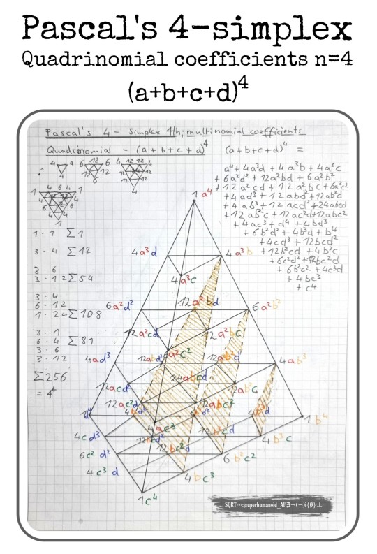
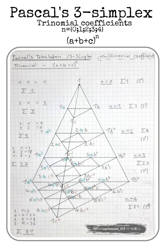
Multinomial coefficients and Pascal's Simplex

For binomials [ (a+b)ⁿ ] the use of Pascal's triangle is helpful. In Pascal's triangle each single row in the triangle defines the coefficients of binomials of each n-value.

For trinomials [ (a+b+c)ⁿ ] this pattern can be extended to a 3-dimensional Pascal's tetrehedron, where each level (and hence a complete triangle) in that tetrehedron defines the coefficients of trinomials of each value of n.

As for quadrinomials [ (a+b+c+d)ⁿ ] the coefficients require an own tetrahedron for each value of n.

[wumblr]

dear seth search multinomial theorem on Wikipedia. as an example for the first question you have as exponents 2,3,5 so the term is 10!/(2!3!5!)*x^3*2^2*y^2*1^5. this makes the right coefficient. expanding a multinomial involves making a term for each permutation of exponents where they must sum to 10 in this case. you can kind of see this in the expansion of a binomial. also i was just saying dont be hard on yourself its difficult to do by yourself and youre making good progress

thank you!! not a whole lot of this makes sense yet but i���m trying to focus on understanding it instead of being mad at the class i’m taking. like, everybody grapples with math, the class doesn’t matter, just keep grappling

sorry i was got defensive, i haven’t been sleeping well and i started worrying that some of these messages were coming from my ex (which is a dumb thing to worry about, really i know they’re not, but there’s always this chance in the back of my mind that he’s checking up on me and waiting for the opportunity to laugh if i fail)

[alihanalihanrin]

Multinomial coefficient

Multinomial coefficient

The polynomial coefficients are the coefficients in the expansion of n {\ properties mapping style value ^ {n}} into monomials x 1 k 1 x 2 k 2 (1 x k 1 x k 2 2). xmkm (x M K) {\ properties display style value x_ not {1} ^ {k_ {1}} x_ not {2} ^ {k_ {2}} \ points x_ not {m} ^ {k_ {m}} }: x 1 + x 2 + ⋯ + xmn = ∑ k 1 (to 1) + k 2 (to 2) + ⋯ + km = nx 1 k 1 x 2 k 2 (to M = N x…

[abhishek21]

Fibonacci Retracement Levels

Let us start with understanding what Fibonacci retracement levels are. So, while defining retracement level, we can say that it is a horizontal line of numbers or price, which indicates the likeliness of support and resistance to occur at a particular time frame. Every level is in line with the percentage. This percentage shows how much percentage the last move has retraced and how likely it will move again. The percentage levels in Fibonacci levels are 23.6%, 38.2%, 61.8% and 78.6%. Sometimes 50% is also used unofficially. These percentage indicators become useful to extract significant points between high and low. Let us assume the share price of a stock is Rs. 10 and drops to 2.36; then it can be said it has retraced to 23.6%, which is a Fibonacci number. Financial traders accept the relevance and importance of Fibonacci numbers in the market.

You might think, who invented this series of percentage patterns in the share market? To answer this, please keep reading. These levels are named after an Italian Mathematician Leonardo Pisano Bigollo, known as Leonardo Fibonacci. The pattern is just named after it because he shared these details with European countries. The actual truth is it was discovered long back in India by an Indian Merchant, and Leonardo learned from him. From ancient times, retirement levels are prevailing in India between 450 and 200 BCE. This retracement pattern has been used in India Since then. Significant work was done on these number systems by great scholars of India. It is believed that great Indian Mathematician Acharya Virahanka has developed Fibonacci Numbers, and the method of sequencing them was found in 600 AD. After the discovery by Acharya Viranhka, many Indian Scholars did more research on that naming, Gopala, Hemachandra, and Narayan Pandita. Pandita found the correlation between Fibonacci numbers and multinomial Coefficients, resulting in the greater usage of Fibonacci Numbers. So, now we are a little clear with what are Fibonacci retracement levels. Let us move ahead with how to calculate Fibonacci retracement levels?

refer our detailed blog to learn more options strategy

[colorgamesblog]

If ???? = ???? = 5, and ??^ = 7?? + 2, what is the correlation coefficient of th

If ???? = ???? = 5, and ??^ = 7?? + 2, what is the correlation coefficient of th

If ???? = ???? = 5, and ??^ = 7?? + 2, what is the correlation coefficient of the data set? Bernoulli, Uniform, Geometric, Binomial, Poisson, Hypergeometric, Negative-Binomial, Multinomial 16. ____________________ Let ?? represent the number of sick people that enters a hospital on Saturday afternoons, for which the average number of sick people arriving is approximately 45.8. 17.…

[endesuch]

If ???? = ???? = 5, and ??^ = 7?? + 2, what is the correlation coefficient of th

If ???? = ???? = 5, and ??^ = 7?? + 2, what is the correlation coefficient of th

If ???? = ???? = 5, and ??^ = 7?? + 2, what is the correlation coefficient of the data set? Bernoulli, Uniform, Geometric, Binomial, Poisson, Hypergeometric, Negative-Binomial, Multinomial 16. ____________________ Let ?? represent the number of sick people that enters a hospital on Saturday afternoons, for which the average number of sick people arriving is approximately 45.8. 17.…

[elaesaturno]

If ???? = ???? = 5, and ??^ = 7?? + 2, what is the correlation coefficient of th

If ???? = ???? = 5, and ??^ = 7?? + 2, what is the correlation coefficient of th

If ???? = ???? = 5, and ??^ = 7?? + 2, what is the correlation coefficient of the data set? Bernoulli, Uniform, Geometric, Binomial, Poisson, Hypergeometric, Negative-Binomial, Multinomial 16. ____________________ Let ?? represent the number of sick people that enters a hospital on Saturday afternoons, for which the average number of sick people arriving is approximately 45.8. 17.…

[ss1986us]

ncert solutions for class 7 maths

class 7 maths

 Foundation of any subject is important specifically when you are taking about maths . maths is important subject for your academic journey and class 7 maths build your interest as well we as solid foundations in the subject in this class you start learning the algebra and its applications . so always take class 7 maths studies seriously . you must be wondering what is the best approach to study class 7 maths ? how to score good marks in class 7 maths ? so to answering to your questions lets discuss the right approach of studying class 7 maths .

 Right approach to study class 7 maths

 About class 7 Books: Selection of right books will help you to have better understanding of the concepts so always make NCERT maths book for class 7 your primary book , follow the sequence of chapters given in NCERT book don’t skip any chapters . after doing NCRET take a reference book or follow entrancei notes which are prepared such a way that it will build your solid foundation in class 7 maths 

About class 7 maths class: Always attend the class in school or in tuitions never skip any class , if you have any work or family function or you are sick plan the missing topic during the holidays and be reedy your topics before the next class. In class listen what teacher wants to explain and make all important points notes in your note book . ask your questions don’t hesitate while asking silly questions in class 7 maths .   

Brief descriptions about Important Chapters covered in class 7 maths

 1. Class 7 maths chapter- NUMBERS

 Natural Numbers: The counting numbers are called Natural Numbers.

          Thus, N = {1, 2, 3, 4, 5,....} is the set of all natural numbers.

Whole Numbers: Whole Numbers are simply the numbers 0, 1, 2, 3, 4, 5, …

           Thus,   W = {0, 1, 2, 3, 4, 5.....} is the set of all Whole Numbers.

Integers: Integers are like whole numbers, but they also include negative numbers ... but still no fractions allowed!

 So, integers can be negative {-1, -2,-3, -4, -5, … }or positive {1, 2, 3, 4, 5, … }, or zer{0}

We can put that all together like this:

              I or Z = { ..., -5, -4, -3, -2, -1, 0, 1, 2, 3, 4, 5, ... }

Rational Numbers: A rational number is a number that can be written as a ratio (p/q form). That means it can be written as a fraction, in which both the numerator (p) and the denominator (q) are integers and q not zero.

The number 8 is a rational number because it     can be written as the fraction 8/1.

Likewise, 3/4 is a rational number because it     can be written as a fraction.

Even a big, clunky fraction like     7,324,908/56,003,492 is rational, simply because it can be written as a     fraction.

 Equivalent rational numbers: Numbers that have the same value but are represented differently.

 2.  Class 7 maths chapter- DIVISIBILITY TESTS, SQUARES, CUBES,SQUARE AND CUBE ROOTS

OVISIBILITY

DIVISIBILITY TEST:

Test of Divisibility by 2 : A number is divisible by 2, if its units digit is any of the digits 0, 2, 4, 6 and 8.

 Example:  Each of the numbers 24, 36, 78, 192, 310, 214166 is divisible by 2.

Prime Factors: A factor of a given number is called a prime factor if this factor is a prime number.

Example: The factors of 42 are 1, 2, 3, 6, 7, 14, 21 and 42. Out of these 2, 3 and 7 are prime numbers. Therefore, 2, 3 and 7 are the prime factors of 42.

 Common Factors: A number which divides each one of the given numbers exactly, is called a common factor of each of the given numbers.

 Example: 4 divide each one of 212 and 356 exactly. Therefore, 4 is a common factor of 212 and 356.

H.C.F. (HIGHEST COMMON FACTOR) OR G.C.D. (GREATEST COMMON DIVISOR) :

 H.C.F. or G.C.D. of two or more numbers is the greatest number that divides each one of them exactly.

 3. Class 7 maths chapter- ALGEBRAIC EXPRESSIONS AND IDENTITIES

 In the previous class, we have learnt about algebraic expressions and their addition and subtraction. In this chapter we shall study multiplication and division of algebraic expressions in the form of monomials and binomials etc.

Constants: A symbol having a fixed numerical value is called a constant.

Variables or Literals: A symbol which takes on various numerical values is known as a variable or a literal.

We know that the perimeter of a square of side a is given by the formula, P = 4a.

Here 4 is a constant, while a and P are variables.

We may give any value to a and get the corresponding value of P.

Algebraic Expressions : A combination of constants and variables, connected by +, - , and is known as an algebraic expression.

Types of algebraic expressions:

 1.           Monomial : An algebraic expression containing only one term, is called a monomial.

2.            Binomial : An algebraic expression containing 2 terms is called a binomial.

3.           Trinomial: An algebraic expression containing 3 terms is called a trinomial.

4.           Multinomial: An algebraic expression containing more than 3 terms, is called a

              multinomial.

Factors of A Term: When numbers and literals are multiple to form a product, then each quantity multiplied is called a factor of the product. A constant factor is called a numerical factor while a variable factor is called a literal factor.

Constant Term: A term of the expression having no literal factor is called the constant term.

Coefficients: Any factor of a term is called the coefficient of the product of other factors.

4. Class 7 maths chapter- EXPONENTS

 INTRODUCTION:

we know that can be written as that is read as two raised to the power three. Similarly, 10 times = , read as three raised to the power ten. In general, if x is any number and m is a positive integer, then we have

m times.

 The number x is called the base and m is called the exponent or the index of the exponential expression.

 5. Class 7 maths chapter- FACTORISATION

Factorisation:

When an algebraic expression can be written as the product of two or more expressions, then each of these expressions is called a factor of the given expression.

 G.C.F. or H.C.F of Monomials: The greatest common factor of given monomials is the common factor having greatest coefficient and highest power of the variables.

G.C.F. or H.C.F of Monomials = (G.C.F. or H.C.F of numerical coefficients)

(G.C.F. or H.C.F of literal coefficients)

 6. Class 7 maths chapter- SETS

 Objects: Everything in this universe, whether living or non living, is called an object. Well-defined collection of objects : A collection of objects is said to be well-defined if itis possible to tell beyond doubt about every object of the universe, whether it is there inour collection or not.

Set :       A well-defined collection of objects is called a set.

              The objects in a set are called its members or elements.

              We usually denote sets by capital letters A, B, C etc.

              If x is an element of a set A, we say that x belongs to A and we write, .

              If x does not belong to A, we write.

              There are two methods of describing a set :

              (i)     Roster Method or Tabulation Method.          

              (ii)    Description Method or Set-builder Form.

 7. Class 7 maths chapter- QUADRATIC EQUATIONS

 Quadratic Equations: A polynomial of degree 2 when equated to zero, gives an equations, called a quadratic equations.

Solving Quadratic Equation:

By solving a quadratic equation, we mean finding its roots.

Zero Product Rule:

If a and b are any two numbers or expressions, then ab = 0 a = 0 or b =0.

    8. Class 7 maths chapter- LINEAR EQUATION IN TWO VARIABLES

 In this chapter we shall we shall learn how to solve linear equations in two variables. For this we shall learn graphical representation of a point in a plane. We shall represent a point with the help of two numbers known as coordinates of that point. The concept of coordinates was given by the French Mathematician Rene Desartes, which integrates Algebra and geometry.

 9.  Class 7 maths chapter-  SPEED, DISTANCE AND TIME

Speed: The rate of change of distance is known as speed.

When an athlete runs a race, the change in the time taken is directly proportional to the change in the distance covered. A change in speed is directly proportional to the change in distance covered. More the speed more is the distance covered in the same time.

Units of Speed: Speed is measured in i) meters/ second or m/s

                                                ii) Kilometers/ hour or km/hr

 10. Class 7 maths chapter- Simple Interest:

                               When money is borrowed, interest is charged for the use of that money for a certain period of time. When the money is paid back, the principal (amount of money that was borrowed) and the interest is paid back. The amount of interest depends on the interest rate, the amount of money borrowed (principal) and the length of time that the money is borrowed.

                             Simple interest is generally charged for borrowing money for short periods of time. Compound interest is similar but the total amount due at the end of each period is calculated and further interest is charged against both the original principal but also the interest that was earned during that period.

                               Interest = Principle x rate of interest x time

   CO

ORDINATE SYSTEM

[udemy-gift-coupon-blog]

Learn Binomial Theorem|concepts and excellent examples-Math ##100%FREEUdemyDiscountCoupons ##realdiscount #Binomial #examplesMath #Excellent #Learn #Theoremconcepts Learn Binomial Theorem|concepts and excellent examples-Math Binomial theorem is an important topic of algebra.Generally many questions do come from this topic in competition exams.This course will be useful for the students who are appearing in class 11th and for those who are preparing for IIT JEE,NDA and MCA entrance exams.The course is useful for both beginners as well as advance level.It covers following areas in details- Binomial Theorem for positive index Properties of Binomial Theorem ,its general term and Middle terms Pascal's Triangle Term from end  Properties of binomial Coefficients Binomial theorem for any index Multinomial theorem and its important results A good number of simple and tough questions have been added here for better understanding of the course and boosting the self confidence of the students. Join now!!!!!! 👉 Activate Udemy Coupon 👈 Free Tutorials Udemy Review Real Discount Udemy Free Courses Udemy Coupon Udemy Francais Coupon Udemy gratuit Coursera and Edx ELearningFree Course Free Online Training Udemy Udemy Free Coupons Udemy Free Discount Coupons Udemy Online Course Udemy Online Training 100% FREE Udemy Discount Coupons https://www.couponudemy.com/blog/learn-binomial-theoremconcepts-and-excellent-examples-math/

[craigbrownphd]

R Packages worth a look

Explore Probability Distributions for Bivariate Temporal Granularities (gravitas) Provides tools for systematically exploring large quantities of temporal data across different temporal granularities (deconstructions of time) by visualizing probability distributions. ‘gravitas’ computes circular, aperiodic, single-order-up or multiple-order-up granularities and advises on which combinations of granularities to explore and through which distribution plots. Bifactor Indices Calculator (BifactorIndicesCalculator) The calculator computes bifactor indices such as explained common variance (ECV), hierarchical Omega (OmegaH), percentage of uncontaminated correlations (PUC), item explained common variance (I-ECV), and more. This package is an R version of the ‘Excel’ based ‘Bifactor Indices Calculator’ (Dueber, 2017) with added convenience features for directly utilizing output from several programs that can fit confirmatory factor analysis or item response models. Ridge-Type Penalized Estimation of a Potpourri of Models (porridge) The name of the package is derived from the French, ‘pour’ ridge, and provides functionality for ridge-type estimation of a potpourri of models. Currently, this estimation concerns that of various Gaussian graphical models from different study designs. Among others it considers the regular Gaussian graphical model and a mixture of such models. The porridge-package implements the estimation of the former either from i) data with replicated observations by penalized loglikelihood maximization using the regular ridge penalty on the parameters (van Wieringen, Chen, 2019) or ii) from non-replicated data by means of the generalized ridge estimator that allows for both the inclusion of quantitative and qualitative prior information on the precision matrix via element-wise penalization and shrinkage (van Wieringen, 2019, ). Additionally, the porridge-package facilitates the ridge penalized estimation of a mixture of Gaussian graphical models (Aflakparast et al., 2018, ). Simulated Maximum Likelihood Estimation of Mixed Logit Models for Large Datasets (mixl) Specification and estimation of multinomial logit models. Large datasets and complex models are supported, with an intuitive syntax. Multinomial Logit Models, Mixed models, random coefficients and Hybrid Choice are all supported. For more information, see Molloy et al. (2019) . http://bit.ly/2TKVw3q

[alihanalihanrin]

Multinomial theorem

Multinomial coefficient

Multinomial coefficients – coefficients in the expansion (x1 + x2 + ⋯ + xm) n by the monomials xk11xk22 … xkmm:

(x1 + x2 + ⋯ + xm) n = ∑k1 + k2 + ⋯ + km = n (nk1 k2 … km) xk11xk22 … xkmm.

The value of the multinomial coefficient (nk1 k2 … km) is determined for all non-negative integers n and k1, k2, …, km such that k1 + k2 + ⋯ + km = n:

(nk1 k2 … km) = n! k1! k2! … km…

[trungtamtiengtrung]

Tiếng Trung chủ đề từ vựng toán học phần 2

Các bạn ạ, mình xin gửi đến các bạn bài viết tiếng Trung chủ đề từ vựng toán học phần 2, ở phần 1 các bạn đã học được hết các từ vựng đó rồi phải không. Kiến thức dưới đây gồm hơn 40 từ vựng mình tổng hợp liên quan đến toán học, các bạn hãy tham khảo và chia sẻ cùng học với bạn bè mình nhé. Chúc các bạn học tập chăm.

Đọc thêm:

>>Tiếng Trung chủ đề từ vựng toán học.

>>Học tiếng Trung đạt hiệu quả cao tại Ngoại ngữ Hà Nội.

Tiếng Trung chủ đề từ vựng toán học phần 2

Danh sách từ vựng tiếng Trung về toán học

截尾 jié wěi     cắt đuôi/ truncation

四舍五入    sìshěwǔrù  làm tròn số/ round

下舍入 xià shě rù    làm tròn xuống/ round down

上舍入 shàng shě rù    làm tròn lên/ round up

代数 dàishù      đại số/ algebra

公式     gōngshì       công thức/ formula, formulae(pl.)

单项式       dānxiàngshì          đơn thức/ monomial

多项式       duōxiàngshì           đa thức/ polynomial, multinomial

系数          xìshù                hệ số/ coefficient

未知数 wèizhīshù        ẩn số/ unknown, x-factor, y-factor, z-factor

等式，方程式     děngshì,  fāngchéngshì     đẳng thức, phương trình/ equation

一次方程     yīcì fāngchéng           phương trình bậc nhất/ simple equation

���次方程          èr cì fāngchéng           phương trình bậc 2/ quadratic equation

运算符 yùnsuàn fú   toán tử/ operator

三次方程        sāncì fāngchéng        phương trình bậc 3/ cubic equation

四次方程         sì cì fāngchéng       phương trình bậc 4/ quartic equation

不等式            bùděngshì       bất đẳng thức/ inequation

对数 duì shù         logarit/ logarithm

指数，幂       zhǐshù      lũy thừa, số mũ/ exponent

乘方 chéng fāng  lũy thừa/ power

二次方，平方 èr cì fāng, píngfāng    phương trình bậc hai, bình phương/ square

三次方，立    sāncì fāng, lì    lập phương/ cube

四次方    sì cì fāng      lũy thừa bậc 4/ the power of four, the fourth power

n次方    lũy thừa bậc n/ the power of n, the nth power

Bạn quan tâm và có nhu cầu học tiếng Trung từ cơ bản đến giao tiếp thành thạo, từ sơ cấp đến trung cấp, HSK 1 đến HSK 5, học giáo trình Hán ngữ 6 quyển, Quyển 1 - quyển 5, hãy xem chi tiết khóa học tiếng Trung tại:

https://ngoainguhanoi.com/trung-tam-hoc-tieng-trung-tot-nhat-tai-ha-noi.html.

开方 kāifāng    khai căn/ evolution, extraction

二次方根，平方根           èr cì fāng gēn, píngfānggēn    căn bậc hai/ square root

阶乘   jiēchéng      giai thừa/ factorial

三次方根，立方根 sāncì fāng gēn, lìfānggēn    căn bậc 3/ cube root

四次方根   sì cì fāng gēn  căn bậc 4/ the root of four, the fourth root

n次方根   n cì fāng gēn     căn bậc n/ the root of n, the nth root

集合      jíhé    tập hợp/ aggregate

元素 yuánsù    nguyên tố/ element

空集 kōng jí     bộ rỗng/ void

子集    zǐ jí      tập hợp con/ subset

补集 bǔ jí      bù/ complement

映射 yìngshè    chiếu/ mapping

函数 hánshù    hàm số/ function

常量      chángliàng    hằng số/ constant

变量       biànliàng    đại lượng biến thiên/ variable

单调性     dāndiào xìng    tính đơn điệu/ monotonicity

图象            tú xiàng     hình ảnh/ image

周期性        zhōuqí xìng         chu kỳ/ periodicity

Các bạn đã lưu lại từ vựng và chia sẻ với những người bạn của mình chưa, hãy thực hành, luyện tập thường xuyên, trau dồi mỗi ngày để có kết quả tốt nhất nào. Chúc các bạn luôn đạt được mục tiêu khi học tiếng Trung. Cố gắng hết sức các bạn nhé.

Nguồn bài viết: trungtamtiengtrung.tumblr.com

[bookpiofficial]

Recursive Computation of Binomial and Multinomial Coefficients and Probabilities | Chapter 07 | Advances in Mathematics and Computer Science Vol. 1

This chapter studies a prominent class of recursively-defined combinatorial functions, namely, the binomial and multinomial coefficients and probabilities. The chapter reviews the basic notions and mathematical definitions of these four functions. Subsequently, it characterizes each of these functions via a recursive relation that is valid over a certain two-dimensional or multi-dimensional region and is supplemented with certain boundary conditions. Visual interpretations of these characterizations are given in terms of regular acyclic signal flow graphs. The graph for the binomial coefficients resembles a Pascal Triangle, while that for trinomial or multinomial coefficients looks like a Pascal Pyramid, Tetrahedron, or Hyper-Pyramid. Each of the four functions is computed using both its conventional and recursive definitions. Moreover, the recursive structures of the binomial coefficient and the corresponding probability are utilized in an iterative scheme, which is substantially more efficient than the conventional or recursive evaluation. Analogous iterative evaluations of the multinomial coefficient and probability can be constructed similarly. Applications to the reliability evaluation for two-valued and multi-valued k-out-of-n systems are also pointed out.  

Author  Details:

Ali Muhammad Ali Rushdi

Department of Electrical and Computer Engineering, King Abdulaziz University, P.O.Box 80204, Jeddah, 21589, Kingdom of Saudi Arabia.

Mohamed Abdul Rahman Al-Amoudi

Department of Electrical and Computer Engineering, King Abdulaziz University, P.O.Box 80204, Jeddah, 21589, Kingdom of Saudi Arabia.

Read full article: http://bp.bookpi.org/index.php/bpi/catalog/view/46/226/386-1

View Volume: https://doi.org/10.9734/bpi/amacs/v1