#u-v graph method

[rajansmoorthy]

Experiment: To Determine the Focal Length of a Convex lens by Plotting Graphs Between u and v and 1/u and 1/v

Focal length of a convex lens: Objective To find the focal length of a convex lens using the lens formula by plotting u and v graph 1/u and 1/v graph Focal length of a convex lens: Apparatus and Material Required Convex lens (let’s assume f=10 cm) Optical bench with 3 uprights (with clamps) Optic needles Meter scale Spirit level  Focal length of a convex lens: Ray Diagram Focal length of a convex…

[softrobotcritics]

Large Language Models and industrial manufacturing, a bibliography

References

Autodesk. (n.d.). Autodesk simulation. Retrieved July 14, 2023, from https://www.autodesk.com/solutions/simulation/overview

Chen, M., Tworek, J., Jun, H., Yuan, Q., de Oliveira Pinto, H. P., Kaplan, J., Edwards, H., Burda, Y., Joseph, N., Brockman, G., Ray, A., Puri, R., Krueger, G., Petrov, M., Khlaaf, H., Sastry, G., Mishkin, P., Chan, B., Gray, S., . . . Zaremba, W. (2021). Evaluating large language models trained on code. ArXiv.https://doi.org/10.48550/arXiv.2107.03374

Christiano, P. F., Leike, J., Brown, T., Martic, M., Legg, S., & Amodei, D. (2017). Deep reinforcement learning from human preferences. In I. Guyon, U. Von Luxburg, S. Bengio, H. Wallach, R. Fergus, S. Vishwanathan, & R. Garnett (Eds.), Advances in neural information processing systems (Vol. 30, pp. 4299–4307). Curran Associates. https://papers.nips.cc/paper_files/paper/2017/hash/d5e2c0adad503c91f91df240d0cd4e49-Abstract.html

Dassault Systèmes. (n.d.). Dassault Systèmes simulation. Retrieved July 14, 2023, from https://www.3ds.com/products-services/simulia/overview/

Dhariwal, P., Jun, H., Payne, C., Kim, J. W., Radford, A., & Sutskever, I. (2020). Jukebox: A generative model for music. ArXiv. https://doi.org/10.48550/arXiv.2005.00341

Du, T., Inala, J. P., Pu, Y., Spielberg, A., Schulz, A., Rus, D., Solar-Lezama, A., & Matusik, W. (2018). InverseCSG: Automatic conversion of 3D models to CSG trees. ACM Transactions on Graphics (TOG), 37(6), Article 213. https://doi.org/10.1145/3272127.3275006

Du, T., Wu, K., Ma, P., Wah, S., Spielberg, A., Rus, D., & Matusik, W. (2021). DiffPD: Differentiable projective dynamics. ACM Transactions on Graphics (TOG), 41(2), Article 13. https://doi.org/10.1145/3490168

Du, Y., Li, S., Torralba, A., Tenenbaum, J. B., & Mordatch, I. (2023). Improving factuality and reasoning in language models through multiagent debate. ArXiv. https://doi.org/10.48550/arXiv.2305.14325

Erez, T., Tassa, Y., & Todorov, E. (2015). Simulation tools for model-based robotics: Comparison of Bullet, Havok, MuJoCo, ODE and PhysX. In Amato, N. (Ed.), Proceedings of the 2015 IEEE International Conference on Robotics and Automation (pp. 4397–4404). IEEE. https://doi.org/10.1109/ICRA.2015.7139807

Erps, T., Foshey, M., Luković, M. K., Shou, W., Goetzke, H. H., Dietsch, H., Stoll, K., von Vacano, B., & Matusik, W. (2021). Accelerated discovery of 3D printing materials using data-driven multiobjective optimization. Science Advances, 7(42), Article eabf7435. https://doi.org/10.1126/sciadv.abf7435

Featurescript introduction. (n.d.). Retrieved July 11, 2023, from https://cad.onshape.com/FsDoc/

Ferruz, N., Schmidt, S., & Höcker, B. (2022). ProtGPT2 is a deep unsupervised language model for protein design. Nature Communications, 13(1), Article 4348. https://doi.org/10.1038/s41467-022-32007-7

Guo, M., Thost, V., Li, B., Das, P., Chen, J., & Matusik, W. (2022). Data-efficient graph grammar learning for molecular generation. ArXiv. https://doi.org/10.48550/arXiv.2203.08031

Jiang, B., Chen, X., Liu, W., Yu, J., Yu, G., & Chen, T. (2023). MotionGPT: Human motion as a foreign language. ArXiv. https://doi.org/10.48550/arXiv.2306.14795

JSCAD user guide. (n.d.). Retrieved July 14, 2023, from https://openjscad.xyz/dokuwiki/doku.php

Kashefi, A., & Mukerji, T. (2023). ChatGPT for programming numerical methods. Journal of Machine Learning for Modeling and Computing, 4(2), 1–74. https://doi.org/10.1615/JMachLearnModelComput.2023048492

Koo, B., Hergel, J., Lefebvre, S., & Mitra, N. J. (2017). Towards zero-waste furniture design. IEEE Transactions on Visualization and Computer Graphics, 23(12), 2627–2640. https://doi.org/10.1109/TVCG.2016.2633519

Li, J., Rawn, E., Ritchie, J., Tran O’Leary, J., & Follmer, S. (2023). Beyond the artifact: Power as a lens for creativity support tools. In Follmer, S., Han, J., Steimle, J., & Riche, N. H. (Eds.), Proceedings of the 36th Annual ACM Symposium on User Interface Software and Technology (Article 47). Association for Computing Machinery. https://doi.org/10.1145/3586183.3606831

Liu, R., Wu, R., Van Hoorick, B., Tokmakov, P., Zakharov, S., & Vondrick, C. (2023). Zero-1-to-3: Zero-shot one image to 3D object. ArXiv. https://doi.org/10.48550/arXiv.2303.11328

Ma, P., Du, T., Zhang, J. Z., Wu, K., Spielberg, A., Katzschmann, R. K., & Matusik, W. (2021). DiffAqua: A differentiable computational design pipeline for soft underwater swimmers with shape interpolation. ACM Transactions on Graphics (TOG), 40(4), Article 132. https://doi.org/10.1145/3450626.3459832

Makatura, L., Wang, B., Chen, Y.-L., Deng, B., Wojtan, C., Bickel, B., & Matusik, W. (2023). Procedural metamaterials: A unified procedural graph for metamaterial design. ACM Transactions on Graphics, 42(5), Article 168. https://doi.org/10.1145/3605389

Mathur, A., & Zufferey, D. (2021). Constraint synthesis for parametric CAD. In M. Okabe, S. Lee, B. Wuensche, & S. Zollmann (Eds.), Pacific Graphics 2021: The 29th Pacific Conference on Computer Graphics and Applications: Short Papers, Posters, and Work-in-Progress Papers (pp. 75–80). The Eurographics Association. https://doi.org/10.2312/pg.20211396

Mirchandani, S., Xia, F., Florence, P., Ichter, B., Driess, D., Arenas, M. G., Rao, K., Sadigh, D., & Zeng, A. (2023). Large language models as general pattern machines. ArXiv. https://doi.org/10.48550/arXiv.2307.04721

Müller, P., Wonka, P., Haegler, S., Ulmer, A., & Van Gool, L. (2006). Procedural modeling of buildings. In ACM SIGGRAPH 2006 papers (pp. 614–623). Association for Computing Machinery. https://doi.org/10.1145/1179352.1141931

Ni, B., & Buehler, M. J. (2024). MechAgents: Large language model multi-agent collaborations can solve mechanics problems, generate new data, and integrate knowledge. Extreme Mechanics Letters, 67, Article 102131. https://doi.org/10.1016/j.eml.2024.102131

O’Brien, J. F., Shen, C., & Gatchalian, C. M. (2002). Synthesizing sounds from rigid-body simulations. In Proceedings of the 2002 ACM SIGGRAPH/Eurographics Symposium on Computer Animation (pp. 175–181). Association for Computing Machinery. https://doi.org/10.1145/545261.545290

OpenAI. (2023). GPT-4 technical report. ArXiv. https://doi.org/10.48550/arXiv.2303.08774

Ouyang, L., Wu, J., Jiang, X., Almeida, D., Wainwright, C., Mishkin, P., Zhang, C., Agarwal, S., Slama, K., Ray, A., Schulman, J., Hilton, J., Kelton, F., Miller, L., Simens, M., Askell, A., Welinder, P., Christiano, P. F., Leike, J., & Lowe, R. (2022). Training language models to follow instructions with human feedback. In S. Koyejo, S. Mohamed, A. Agarwal, D. Belgrave, K. Cho, & A. Oh (Eds.), Advances in Neural Information Processing Systems (Vol. 35, pp. 27730–27744). Curran Associates. https://proceedings.neurips.cc/paper_files/paper/2022/hash/b1efde53be364a73914f58805a001731-Abstract-Conference.html

Özkar, M., & Stiny, G. (2009). Shape grammars. In ACM SIGGRAPH 2009 courses (Article 22). Association for Computing Machinery. https://doi.org/10.1145/1667239.1667261

Penedo, G., Malartic, Q., Hesslow, D., Cojocaru, R., Cappelli, A., Alobeidli, H., Pannier, B., Almazrouei, E., & Launay, J. (2023). The RefinedWeb dataset for Falcon LLM: Outperforming curated corpora with web data, and web data only. ArXiv. https://doi.org/10.48550/arXiv.2306.01116

Prusinkiewicz, P., & Lindenmayer, A. (1990). The algorithmic beauty of plants. Springer Science & Business Media.

Radford, A., Wu, J., Child, R., Luan, D., Amodei, D., & Sutskever, I. (2019, February 14). Language models are unsupervised multitask learners. OpenAI. https://openai.com/index/better-language-models/

Ramesh, A., Pavlov, M., Goh, G., Gray, S., Voss, C., Radford, A., Chen, M., & Sutskever, I. (2021). Zero-shot text-to-image generation. Proceedings of Machine Learning Research, 139, 8821–8831. https://proceedings.mlr.press/v139/ramesh21a.html

Repetier. (n.d.). Repetier software. Retrieved July 20, 2023, from https://www.repetier.com/

Richards, T. B. (n.d.). AutoGPT. Retrieved February 11, 2024, from https://github.com/Significant-Gravitas/AutoGPT

Rozenberg, G., & Salomaa, A. (1980). The mathematical theory of L systems. Academic Press.

Slic3r. (n.d.). Slic3r - Open source 3D printing toolbox. Retrieved July 20, 2023, from https://slic3r.org/

Stiny, G. (1980). Introduction to shape and shape grammars. Environment and Planning B: Planning and Design, 7(3), 343–351. https://doi.org/10.1068/b070343

Sullivan, D. M. (2013). Electromagnetic simulation using the FDTD method. John Wiley & Sons. https://doi.org/10.1002/9781118646700

Todorov, E., Erez, T., & Tassa, Y. (2012). MuJoCo: A physics engine for model-based control. In 2012 IEEE/RSJ International Conference on Intelligent Robots and Systems (pp. 5026–5033). IEEE. https://doi.org/10.1109/IROS.2012.6386109

Turing, A. M. (1936). On computable numbers, with an application to the Entscheidungsproblem. Proceedings of the London Mathematical Society, s2-42(1), 230–265. https://doi.org/10.1112/plms/s2-42.1.230

Willis, K. D., Pu, Y., Luo, J., Chu, H., Du, T., Lambourne, J. G., Solar-Lezama, A., & Matusik, W. (2021). Fusion 360 gallery: A dataset and environment for programmatic CAD construction from human design sequences. ACM Transactions on Graphics (TOG), 40(4), Article 54. https://doi.org/10.1145/3450626.3459818

Xu, J., Chen, T., Zlokapa, L., Foshey, M., Matusik, W., Sueda, S., & Agrawal, P. (2021). An end-to-end differentiable framework for contact-aware robot design. ArXiv. https://doi.org/10.48550/arXiv.2107.07501

Yu, L., Shi, B., Pasunuru, R., Muller, B., Golovneva, O., Wang, T., Babu, A., Tang, B., Karrer, B., Sheynin, S., Ross, C., Polyak, A., Howes, R., Sharma, V., Xu, P., Tamoyan, H., Ashual, O., Singer, U., . . . Aghajanyan, A. (2023). Scaling autoregressive multi-modal models: Pretraining and instruction tuning. ArXiv.https://doi.org/10.48550/arXiv.2309.02591

Zhang, Y., Yang, M., Baghdadi, R., Kamil, S., Shun, J., & Amarasinghe, S. (2018). GraphIt: A high-performance graph DSL. Proceedings of the ACM on Programming Languages, 2(OOPSLA), Article 121. https://doi.org/10.1145/3276491

Zhao, A., Xu, J., Konaković-Luković, M., Hughes, J., Spielberg, A., Rus, D., & Matusik, W. (2020). RoboGrammar: Graph grammar for terrain-optimized robot design. ACM Transactions on Graphics (TOG), 39(6), Article 188. https://doi.org/10.1145/3414685.3417831

Zilberstein, S. (1996). Using anytime algorithms in intelligent systems. AI Magazine, 17(3), 73–83. https://doi.org/10.1609/aimag.v17i3.1232

[shkspr]

1/2 i think ill be able to list all of them but im not sure so i will try? the eye, the web, the hunt, the flesh, corruption, the vast, the buried, the stranger, the spiral, the dark, desolation, the lonely, the end, extinction technically. this took me some time tho and i still am missing one bc i know that there are 14 (15 with extinction)

2/2 and for the method. entities usually come in pairs or at least i associate them this way (for example vast and buried being opposites or spiral and stranger being similar, hunt and flesh also feel like a pair to me even though it doesnt really make sense) also im thinking of any meta theory graphs ive seen or trying to remember avatars/statements

thats valid and makes a lot of sense!! the 1 u forgot was the slaughter which is understandable lol. i remember them in little groups too but not grouped conceptually just grouped alphabetically bc its easy for me to remember like. B-C-2D-3E-F-H-L and then theres a big jump in the alphabet and it goes to 3S-V-W and thats all of em. also i like to automatically count the extinction bc it saves me from the confusion of like listing it and then counting 14 and thinking thats all of them when i actually forgot one of the others and replaced it w the extinction

[transannabeth]

im in ap bio and our teacher doesn’t actually teach us anything but he gives us 9 page packets to fill out during the unit (which is like. 4 classes?) and literally every single question aside from graphs or labeling images is on quizlet so we use that and now we’re all gonna fail our ap exam

ahhhhhhhhhhh!!!!!!!!!!!!!!!!

god that sounds a w f u l !!!! but i also know that that is the experience of a lot of kids who take ap bio and it sucks!!! bio is super super interesting if you have a teacher who’s methods aline with your learning style and is just genuinely really excited to teach it. i still remember lots of random things about hormones or cell processes just because of how my teacher taught them

if you want some genuine recommendations from me, i always recommend the review book. it’s basically your textbook but without a lot of the language that makes it hard to understand. it’s just super streamlined and i would use it to study before each individual test, not just the ap exam. it’s so much more straightforward and i found that really helps and it also has practice problems and answers*

other than that i recommend crash course and bozeman science on youtube. crash course is (obviously) a crash course, so it’s not as detailed, but i really like using it for overviews. if i don’t really remember or understand something hank mentions, i know that it’s something i need to look at again. and then i always would listen to it as i fell asleep and all morning the day before tests, because i just really really hoped that would just. help. bozeman science is (in my opinion) a lot more boring, but they’re specifically made for the ap course and exam and are a lot more detailed. if you’re really struggling, i recommend those**

i’m sorry your teacher sucks :// i really do genuinely believe that way more people would love biology if they just had a better teacher. but hey, don’t give up the ap just yet! you’ve got time! (don’t bother studying plants. no one cares about plants)

[footnotes below cut cause i don’t shut up]

*btw this is true of all the ap books i ever used. i highly recommend them for sciences and history, and as much as i still didn’t understand calculus, i understood it a tiny bit more and it helped to be able to see what felt really really confusing simplified on a page. it’s just the barebones knowledge and i know for me, it’s so much easier to process and figure out what you need to know. i really wish all textbooks were written the way the review books were honestly

**i apply the same principal to both world and us ap history. crash course videos are VERY good for basic overview and finding holes in your knowledge. i also would put it on in the background as i reviewed other notes or read my review book because i was like “this is a ridiculous amount of information, maybe i should just like surround myself in a bubble of it” (i have no idea if it helped). and then for the more thorough videos, i would check out joczproductions, also on youtube. they’re longer and kind of boring but they’re good for like. getting a lot of information at once. AND there are videos that compare different areas and themes and whatnot which are REALLY important to keep in mind on the exam!!!

(also if you google ‘apush notes site’..............)

(i l o v e amsco review book for apush btw, it doesn’t have answers for the practice questions but like i really do love it and have genuinely considered buying a new copy, i gave mine away, just to have to read through. for other books, i looked at both the official college board ones and other unofficial versions. for those just go with whatever looks like it’ll help you more, for my ap psych book i literally just went back and forth between two different review books because i hated the textbook that much)

[hometuitionorg]

1. To determine resistivity of two / three wires by plotting a graph between potential difference versus current.

2. To find resistance of a given wire / standard resistor using metre bridge.

OR

To verify the laws of combination (series) of resistances using a metre bridge.

OR

To verify the Laws of combination (parallel) of resistances using a metre bridge.

3. To compare the EMF of two given primary cells using potentiometer.

OR

To determine the internal resistance of given primary cell using potentiometer.

4. To determine resistance of a galvanometer by half-deflection method and to find its figure of merit.

5. To convert the given galvanometer (of known resistance and figure of merit) into a voltmeter of desired range and to verify the same.

OR

To convert the given galvanometer (of known resistance and figure of merit) into an ammeter of desired range and to verify the same.

6. To find the frequency of AC mains with a sonometer.

Experiments Assigned for Term-II

1. To find the focal Length of a convex lens by plotting graphs between u and v or between 1/u and 1/v.

2. To find the focal Length of a concave lens, using a convex lens.

or,

To find the focal length of a convex mirror, using a convex Lens

3. To determine angle of minimum deviation for a given prism by plotting a graph between angle of incidence and angle of deviation.

4. To determine refractive index of a glass slab using a travelling microscope.

5. To find refractive index of a liquid by using convex Lens and plane mirror.

6. To draw the I-V characteristic curve for a p-n junction in forward bias and reverse bias.

_______________________________

#isc #icse #icsevscbse #icsememes #education #likeforlikes #like4likes #likesforlike #likeforfollow #liketime #likeforlikeback #likelike #likers #likeme #followforfollowback #follow #follow4followback #followers #followｍe #friends #study #instadaily #instagram #instagood #instalike #insta #instamood #instaphoto #instacool #india 📖📖📖📖

[medalmonkey]

Board practical exam paper

All India Senior Secondary Certificate Exam (2020 – 21) SUB: PHYSICS (042)

Date: …………                                                                  Time: 03hrs

Section A

 1.      To determine resistivity of two/three wires by plotting a graph for potential difference versus current.

2.      To find resistance of a given wire/ standard resistor using meter bridge.

3.      To determine resistance of a galvanometer by half-deflection method and to find its figure of merit.

4.      To convert the given galvanometer (of known resistance and figure of merit) into a voltmeter of desired range and to verify the same.

 Section B

 1.      To find the focal length of a convex lens by plotting graphs between u and v or between 1/u and 1/v.

2.      To find the focal length of a convex mirror, using a convex lens.

3.      To determine angle of minimum deviation for a given prism by plotting a graph between angle of incidence and angle of deviation.

4.      To draw the I-V characteristic curve for a p-n junction diode in forward bias and reverse bias.

 Evaluation Scheme:

o   Tow experiments one from each section                         8+8 marks

o   Practical record (experiments and activities)                      7 marks

o   Viva based on experiments                                                 7 marks

Total marks                                                                           30 marks 

    Internal examiner signature           External examiner signature

[zombiepineapple]

Game Theory (SSG) in Physical and Cybersecurity

Most organizations only have so many resources to go around, forcing them to choose where and when to use their money and assets to improve security. In the past, this forced the cyber community to develop different methods and routes to best keep businesses safe. These were algorithmic game theories that need to be tested, leading to what we know today as “cyber games” (Sinha, et al.). Many of us have heard of the Red Team versus Blue Team events or a company hiring a security group to mock attack or break in. Even Disaster Recovery table top games are reminiscent of a kind of play, like cards or escape rooms.

Here are some of these algorithms that helped randomize and strengthen security: ARMOR, IRIS, Protect, Trusts, Paws, and Midas. These, specifically, were all used for physical security in some way. Usually to randomize patrol units or protect wildlife. Using these algorithms in cybersecurity is relatively new but have already been used for “deep packet inspection, optimal use of honey pots, and enforcement of privacy policies” (Sinha, et al.; Vanek O, Yin Z, Jain M, et al.; Dukota K, Lisy V, Kiekintveld C, et al.; Blocki J, Christin N, Datta A, et al.).

Sometimes you may see these games called “Stackelberg Security Games” or SSG. This is when one side has to protect something and the other has to use adversarial reasoning to try to invade, destroy, or defeat. The article I read explains more on research conducted on the results of these games as well as challenges in doing this research and real-world difficulties. For example, when you sit down to play a game and you’re given three options, you’re going to try to go with the best option. A real-world challenge is that humans don’t always pick the best option, especially under pressure or time-crunch and especially when they’re in an emergency situation. So, since no one is perfect, these games simply ask: Is this a better security profile than before (Sinha, et al.)?

Most of these algorithms rely on organizations following them for timing. For example, they compared how well a metro in Los Angeles ran based off a human-made schedule versus an algorithmically designed one. Humans taking the metro gave their opinions on their ride experience, not knowing which had made the schedule for the day. Not only did the algorithm win, but letting a computer do that work saves a human employee, on average, an entire day’s worth of work creating the schedule (Sinha, et al.)!

Another example is using these algorithms to pick and inspect data packets in an extremely large network, as if taking a random survey sample. A network can’t be expected to “deep dive” into every single data packet that hops to or from a device, so we’re back to a limited allocation of resources.

Game theory to the rescue: “The objective of the defender is to prevent the intruder from succeeding by selecting the packets for inspection, identifying the attacker, and subsequently thwarting the attack … The authors provide polynomial time approximation algorithm that benefits from the submodularity property of the discretized zero-sum variant of the game and finds solutions with bounded error in polynomial time (Sinha, et al.).”

That’s pretty technical but basically means that the game will help the company playing it decide how often they need to set up their system to do these random checks. For example, PetCo may only have to check once an hour, while PetSmart might have to set their system to check a random data packet every minute.

Most people think physical and cybersecurity are different, but they have a lot of common ground. The largest being that a computer algorithm can help when time and assets are tight!

Resources

Blocki J, Christin N, Datta A et al. Audit games. In: Proceedings of the 23rd International Joint Conference on Artificial Intelligence, 2013.

Durkota K, Lisy V, Kiekintveld C et al. Game-theoretic algorithms for optimal network security hardening using attack graphs. In: Proceedings of the (2015) International Conference on Autonomous Agents and Multiagent Systems. AAMAS '15, 2015. Richland, SC: International Foundation for Autonomous Agents and Multiagent Systems (IFAAMAS).

Sinha, Arunesh, et al. "From physical security to cybersecurity." Journal of Cybersecurity, 2015, p. 19+. Gale OneFile: Computer Science, link.gale.com/apps/doc/A468772624/CDB?u=lirn55593&sid=CDB&xid=435a0a02. Accessed 22 Apr. 2021.

Vanek O, Yin Z, Jain M et al. Game-theoretic resource allocation for malicious packet detection in computer networks. In: Proceedings of the 11th International Conference on Autonomous Agents and Multiagent Systems (AAMAS), 2012. Richland, SC: International Foundation for Autonomous Agents and Multiagent Systems (IFAAMAS).

[skillele]

Baseline to Measurement

I completed the same tasks for my first measurement that I did for my baseline performance. This included the two strumming patterns and the chord progression. Although, I noticed that for my baseline I played Fadd9 instead of Am. This mix-up ended up helping me in the long run (more on that later). When practicing, I decided that playing to a song helped me with knowing when to switch a chord. So I tried this out with the chorus of “House of Gold” (vocals only). I set the playback speed to .75, which was a good starting speed for me.

Practice: After a week of practicing, I noticed that I was starting to gain anticipatory behaviors while playing. For example, if I was playing F to G, while playing F I would look at the chords that form G. Additionally, I would think about the positioning of my fingers on the G chord. This was a highlighting moment in my practice time, because it was some sort of evidence that I was retaining something out of this practice. My ultimate goal is to flow and become fluid in every aspect of learning to play ukulele and this gave me a little confidence and proof that it’s possible. I think that’s a crucial factor in learning any skill, having the motivation to pick it up, but also keeping that motivation when no progress (or interesting progress) is shown. 

As far as the mistake in practicing the wrong four chords I mentioned earlier, this helped my methods in diminishing some practice/order effects in playing the same four chords in the same order. My first measurement includes the same four chords, but my practice with the song switches up the order and replaces a chord (remember Am—>Fadd9). On a side note, Fadd9 is still a beginner chord, here’s a video that provides some explanation: https://www.youtube.com/watch?v=8zOgwD-TQME. 

Measurement: I followed the same procedure as baseline when measuring my first performance level by recording myself playing the chord progression with the strumming pattern (with all fingers and then just thumb): D-D-U-U-D-U. This pattern was executed 2x for each chord.

My initial goal in the semester was to work on my strumming, however I got the hang of it more quickly than I had anticipated--moving from a simple down strum to the D-D-U-U-D-U pattern. So I felt like my next goal was to get comfortable with the fret side of the uke. This would include the motor movement involved in forming my fingers into the correct chords, pressing down on the strings (with enough pressure), and switching between chords with ease. I struggled with these areas the most at baseline, so I felt they were most appropriate to measure. I decided to count the total errors of the whole session and separated the errors into three groups: dead notes, finger pressure, finger placement/adjustment.

Here’s a graph comparing errors at baseline and the first measurement:

I also have a graph of completion time for each session:

Note: I did not focus on timing for this first performance session since that wasn’t part of my goal, however I wanted to note that it took slightly less time for me to do the same task a week later. 

Thoughts on improvement:

Pros: I enjoyed my new technique of playing chords in a song with the vocals included. I find that knowing the words to a song helps with knowing what notes to produce and timing (for when I start to practice that). Overall my measurement session felt less “calculated” when it came to decision-making. I felt like my chord switches and strumming were a bit more fluid compared to baseline. I think I have gotten a lot better at the motor aspect. One major change I have noticed is my shift in hand position. I find myself slanting my fingers so that I don’t touch other strings that results in a buzzing or dead note sound. 

Cons: I am feeling a little uncomfortable with my wrist after playing for awhile and I’m not sure if it is from this shift I am making. I also notice that I’m sometimes using my thumb to hold up the ukulele when I make these shifts. I know that people play in a way that’s comfortable for them, however there is a standard posture that a ukulele player should adopt. They say there’s a YouTube video for everything, so I plan to find a few to help fix elements relating to posture.

[dailynewswebsite]

Will it be a ‘V’ or a ‘K’? The many shapes of recessions and recoveries

A 'V' restoration is seen as the easiest way to bounce again from a recession. Steve Stone/Second through Getty Photos

Recessions – sometimes outlined as two consecutive quarters of declining financial output – are at all times painful when it comes to how they have an effect on our financial well-being. Like all unhealthy issues, luckily, they finally finish and a restoration begins.

However not all recoveries or recessions look the identical. And economists tend to check their various paths with letters of the alphabet.

For instance, through the present state of affairs, you could have the heard the path the restoration may take in contrast with a “V,” a “W” or perhaps a “Okay.”

As a macroeconomist, I do know this alphabet soup might be complicated for a lay reader. So right here’s a information to among the mostly used letters.

‘V’ for victory

Whereas recessions are by no means a superb factor, the “V-shaped” restoration is deemed the best-case situation. In a recession with a V form, the decline is fast, however so is the restoration.

instance of this kind of recession happened in 1981 and 1982. That recession occurred after then-Federal Reserve Chair Paul Volcker quickly raised rates of interest starting in 1979 in an effort to curb excessive inflation. This triggered a pointy recession – resulting in what was then the very best unemployment charge within the U.S. because the Nice Despair.

However outdoors of financial circles, this recession is little remembered. Why? Primarily as a result of the restoration was so fast. After Volcker started slicing rates of interest within the second half of 1982, the economic system entered a restoration as sharp because the recession.

‘U’ and a protracted backside

Conversely, a “U-shaped” recession usually has an extended period, each for the downturn and the restoration interval. The 2001 recession that adopted the dot-com bubble and the 9/11 assaults suits into this class.

In some methods, the post-dot-com recession was a light one. The autumn in employment from the job market’s peak in February 2001 till the trough in August 2003 was solely barely lower than 2%. But it took over two years of decline for the economic system to backside out, and it took one other yr and a half for the variety of jobs to exceed the pre-recession peak. Moreover, the period of time spent close to the underside of the recession was comparatively lengthy.

The reclining ‘L’

The final U.S. recession, which coincided with the monetary disaster of 2008, was particularly brutal.

Economists name it an “L-shaped” recession as a result of there was an preliminary sharp downturn, however a really plodding restoration. To see the L, you should think about the letter type of reclining backward on its finish.

The economic system declined quickly after the September 2008 failure of Lehman Brothers, and employment plunged about 6.3% from its pre-recession peak earlier than reaching its low level. The tempo of job creation within the restoration was very sluggish. It took nearly 4½ years to get better all the roles misplaced.

‘Okay’ and a two-track restoration

It might be onerous to see how a Okay might be utilized to information on a graph, but it surely’s the letter more and more getting used to explain the trail of the present recession and eventual restoration.

Fed Chair Jerome Powell didn’t name it a “Okay” however that’s principally what he meant when he mentioned the present financial trajectory in a latest handle. He expressed considerations that the U.S. will expertise a “two-track restoration” wherein issues get higher rapidly for some folks, whereas staying unhealthy for others.

Is that the form of recession we’re in?

It’s unclear. Thus far, wanting on the entire economic system, the U.S. has what has been referred to as a “checkmark” or “swoosh” recession. It started to look one thing like a V, with a pointy drop in employment after which the beginnings of a fast enhance. However that restoration has begun to stall – although not for everybody.

[Deep knowledge, daily. Sign up for The Conversation’s newsletter.]

As Powell advised, the restoration may look totally different to numerous teams. White-collar staff may even see a “V,” as their jobs are extra able to being achieved remotely. Blue-collar staff are seeing one thing nearer to a U or L. One evaluation exhibits that medium- to high-wage staff have gained again nearly all the roles misplaced through the shutdown earlier this close to. Conversely, employment of lower-wage staff remains to be greater than 20% under its pre-COVID-19 peak.

Recessions are powerful for anybody to dwell via. Nevertheless, the form of the restoration could make it roughly bearable.

William Hauk ne travaille pas, ne conseille pas, ne possède pas de elements, ne reçoit pas de fonds d'une organisation qui pourrait tirer revenue de cet article, et n'a déclaré aucune autre affiliation que son organisme de recherche.

from Growth News https://growthnews.in/will-it-be-a-v-or-a-k-the-many-shapes-of-recessions-and-recoveries/ via https://growthnews.in

[ohaithe-re]

The "dichotomy theorem" is a statement about finding homomorphisms between graphs. A homomorphism from a graph G to a graph H is a function f : V(G) -> V(H), so that f(u) and f(v) are neighbors whenever u and v are neighbors. For example: if H has a vertex p that is its own neighbor, a self-loop, then you could map every vertex in G to p. Since f(u) = p = f(v), and p is its own neighbor, this trivially satisfies the requirements. Another example is when H = K3, a triangle. We can call these three vertices r, g, and b. Now finding a homomorphism f means mapping each vertex to one of these three "colors", [r]ed [g]reen or [b]lue. If two vertices in G are neighbors, then applying f to that pair has to give two different colors. So, finding a homomorphism from G to K3 is equivalent to finding a 3-coloring of G.

The dichotomy theorem states that for any fixed H, the problem of "Given G, is there a homomorphism from G to H?" is either in P or is NP-Complete. This is a deep theorem, and wasn't proved until 2017, with pretty advanced methods. A not-so-hard extension of this is that any "finite constraint problem", like 3-SAT, or a set of bounded-size equations over a finite field, is also necessarily either P or NP-Complete. This is shown by establishing a polynomial-time computable equivalence between a constraint problem and an appropriate graph homomorphism problem, such that either can always be written in terms of the other.

As nice and broad as this result is, it doesn't capture the problem of graph isomorphism, which is not known to be P or NP-Complete. This problem can also be naturally phrased in terms of graph homomorphisms: given two graphs G and H, are there graph homomorphisms f1 : G -> H, and f2 : H -> G, such that f1 is the inverse of f2? There is no known way to encode graph isomorphism as a constraint problem, though. In the same way that many constraint problems can be described by a graph homomorphism problem to a fixed graph, many isomorphism problems (of different structures) can be described by a graph isomorphism problem.

I'm trying to figure out if there's a natural problem space that captures both constraint problems and isomorphism problems, that could permit a "trichotomy theorem" kind of thing, where everything is either P or NP-Complete or GI-complete (graph-isomorphism complete). An interesting candidate space I thought of would be a sort of 'graph category completion' problem. You're given a small category of graphs, where some are fixed and some are part of the parameters of the problem, and your goal is to find a set of graph morphisms that satisfy given relations. So a constraint problem would be:

Category with 2 objects G and H, H is fixed, G is part of the problem, one morphism f : G -> H, no relations.

and a graph isomorphism problem would be:

Category with 2 objects G and H, none are fixed, G and H are part of the problem, two morphisms f1 : G -> H and f2 : H -> G, relations are that f1∘f2=id_G, and f2∘f1=id_H.

One more important example is:

Two objects G and H, H is fixed, and you want a morphism f from H to G. This problem is always in P, because you can enumerate all potential functions f in time O( |G| ^ |H| ). Since |H| is a constant, this polynomial time.

And then the question is, is any such "find the morphisms" problem necessarily either P/NP-Complete/GI-Complete? For most of the simple categories I can think of, I could pretty quickly show it was one of these three. Here's a more complicated example:

Category with four objects: {P, H, G1, G2}; P and H are fixed; G1 and G2 are part of the problem; six morphisms {h1 : H->G1,  g1 : G1 -> G2,  g2 : G2 -> G1,   h2 : G2 -> H,  p1 : P -> H,  p2 : H -> P}; relations are {g2∘g1=id_G1,  g1∘g2=id_G2,  h2∘g1∘h1 = p1∘p2}.

That's a long statement, so let me explain why it's interesting -- I also have a picture attached above. The composition p1∘p2 is going to be some endomorphism of H, so, not necessarily an isomorphism, or the identity. The laws relating g1 and g2 mean that G1 is isomorphic to G2. Then instead of finding h2, we can define a new morphism h3 : G1 -> H, where h3 = h2∘g1. So now we're finding endomorphisms of H given by h3∘h1 and p1∘p2, that go through G1 and P respectively. If we have found any 4 morphisms h3, h1, p1, and p2, that don't necessarily satisfy the laws we want, we can define new ones: h1' = h1∘p1∘p2, and p1' = h3∘h1∘p1. Now h3∘h1' = h3∘h1∘p1∘p2 = p1'∘p2, and so these new morphisms will satisfy the laws. So we find these morphisms in polynomial time since |H| is a constant (or reject if we fail), and then we're left with finding an isomorphism between G1 and G2, so the whole thing is GI-complete.

This general strategy of diving up the category into isomorphism-like subproblems (GI-complete), and problems of finding morphisms from a fixed structure to a graph (which are P-time), seems to address most cases. I wonder how hard it would be hard to prove this works in general. Any reasonable proof would certainly use the normal dichotomy theorem as a giant hammer.

Some things I'm wondering about, as a potentially interesting thing to allow in this "category completion" problem:

"Morphism f is faithful", i.e. f(u) and f(v) are neighbors only if u and v are neighbors

"Morphism f is injective" / "Morphism f is surjective".

Filling in a category with new graphs. Instead of just having to solve for morphisms, now finding objects is also part of the problem. Without putting bounds on the size of the "answer" graph, it's not immediately clear that the resulting problem is even in NP. I suspect you could show that it's always at most the product of the sizes of the other graphs given, or something like that, which would suffice to put it in NP.

[the-grendel-khan]

Letter to an interested student.

I had the good luck to chat with a high-school student who was interested in doing the most good she could do with hacker skills. So I wrote the letter I wish someone had written me when I was an excitable, larval pre-engineer. Here it is, slightly abridged.

Hi! You said you were interested in learning IT skills and using them for the greater good. I've got some links for learning to code, and opportunities for how to use those skills. There's a lot to read in here--I hope you find it useful!

First, on learning to code. You mentioned having a Linux environment set up, which means that you have a Python runtime readily available. Excellent! There are a lot of resources available, a lot of languages to choose from. I recommend Python--it's easy to learn, it doesn't have a lot of sharp edges, and it's powerful enough to use professionally (my current projects at work are in Python). And in any case, mathematically at least, all programming languages are equally powerful; they just make some things easier or more difficult.

I learned a lot of Python by doing Project Euler; be warned that the problems do get very challenging, but I had fun with them. (I'd suggest attempting them in order.) I've heard good things about Zed Shaw's Learn Python the Hard Way, as well, though I haven't used that method to teach myself anything. It can be very, very useful to have a mentor or community to work with; I suggest finding a teacher who's happy to help you with your code, or at the very least sign up for stackoverflow, a developer community and a very good place to ask questions. (See also /r/learnprogramming's FAQ.) The really important thing here is that you have something you want to do with the skills you want to learn. (As it is written, "The first virtue is curiosity. A burning itch to know is higher than a solemn vow to pursue truth.") Looking at my miscellaneous-projects directory on my laptop, the last thing I wrote was a Python script to download airport diagrams from the FAA's website (via some awful screenscraping logic), convert them from PDFs to SVGs, and upload them to Wikimedia Commons. It was something I was doing by hand, and then I automated it. I've also used R (don't use R if you can help it; it's weird and clunky) to make choropleth maps for internet arguments, and more Python to shuffle data to make Wikipedia graphs. It's useful to think of programming as powered armor for your brain.

You asked about ethical hacking. Given that the best minds of my generation are optimizing ad clicks for revenue, this is a really virtuous thing to want to do! So here's what I know about using IT skills for social good.

I mentioned the disastrous initial launch of healthcare.gov; TIME had a narrative of what happened there; see also Mikey Dickerson (former SRE manager at Google)'s speech to SXSW about recruiting for the United States Digital Service. The main public-service organizations in the federal government are 18F (a sort of contracting organization in San Francisco) and the United States Digital Service, which works on larger projects and tries to set up standards. The work may sound unexciting, but it's extraordinarily vital--veterans getting their disability, immigrants not getting stuck in limbo, or a child welfare system that works. It's easy to imagine that providing services starts and ends with passing laws, but if our programs don't actually function, people don't get the benefits or services we fought to allocate to them. (See also this TED talk.)

The idea is that most IT professionals spend a couple of years in public service at one of these organizations before going into the industry proper. (I'm not sure what the future of 18F/USDS is under the current administration, but this sort of thing is less about what policy is and more about basic competence in executing it.)

For a broader look, you may appreciate Bret Victor's "What Can a Technologist Do About Climate Change?", or consider Vi Hart and Nicky Case's "Parable of the Polygons", a cute web-based 'explorable' which lets you play with Thomas Schelling's model of housing segregation (i.e., you don't need actively bitter racism in order to get pretty severe segregation, which is surprising).

For an idea of what's at stake with certain safety-critical systems, read about the Therac-25 disaster and the Toyota unintended-acceleration bug. (We're more diligent about testing the software we use to put funny captions on cat pictures than they were with the software that controls how fast the car goes.) Or consider the unintended consequences of small, ubiquitous devices.

And for an example of what 'white hat' hacking looks like, consider Google's Project Zero, which is a group of security researchers finding and reporting vulnerabilities in widely-used third-party software. Some of their greatest hits include "Cloudbleed" (an error in a proxying service leading to private data being randomly dumped into web pages en masse), "Rowhammer" (edit memory you shouldn't be able to control by exploiting physical properties of RAM chips), and amazing bug reports for products like TrendMicro Antivirus.

To get into that sort of thing, security researchers read reports like those linked above, do exercises like "capture the flag" (trying to break into a test system), and generally cultivate a lateral mode of thinking--similar to what stage magicians do, in a way. (Social engineering is related to, and can multiply the power of, traditional hacking; Kevin Mitnick's "The Art of Deception" is a good read. He gave a public talk a few years ago; I think that includes his story of how he stole proprietary source code from Motorola with nothing but an FTP drop, a call to directory assistance and unbelievable chutzpah.)

The rest of this is more abstract, hacker-culture advice; it's less technical, but it's the sort of thing I read a lot of on my way here.

For more about ethical hacking, I'd be remiss if I didn't mention Aaron Swartz; he was instrumental in establishing Creative Commons licensing, the RSS protocol, the Markdown text-formatting language, Reddit and much else. As part of his activism, he mass-harvested academic journal articles from JSTOR using a guest account at MIT. The feds arrested him and threatened him with thirty-five years in prison, and he took his own life before going to trial. It's one of the saddest stories of the internet age, I think, and it struck me particularly because it seemed like the kind of thing I'd have done, if I'd been smarter, more civic-minded, and more generally virtuous. There's a documentary, The Internet's Own Boy, about him.

Mark Pilgrim is a web-standards guy who previously blogged a great deal, but disappeared from public (internet) life around 2011. He wrote about the freedom to tinker, early internet history, long-term preservation (see also), and old-school copy protection, among other things.

I'll leave you with two more items. First, a very short talk, "wat", by Gary Bernhardt, on wacky edge cases in programming language. And second, a book recommendation. If you haven't read it before, Gödel, Escher, Bach is a wonderfully fun and challenging read; it took me most of my senior year of high school to get through it, but I'd never quite read anything like it. It's not directly about programming, but it's a marvelous example of the hacker mindset. MIT OpenCourseWare has a supplemental summer course (The author's style isn't for everyone; if you do like it, his follow-up Le Ton beau de Marot (about language and translation) is also very, very good.)

I hope you enjoy; please feel free to send this around to your classmates--let me know if you have any more specific questions, or any feedback. Thanks!

[journeythroughbible]

As we Coron-on

To explain my “humor” ... “ Coron-on” is to “Drone-on” with Corona-virus blues.

I have taken a few weeks off from commenting about this “pandemic.” But the first thing is to let us look at the numbers for today 7/6/20; total cases are 11,483,400, with 534,938 total deaths. In the USA, we have 2,288,915 cases, with 130,007 deaths. The percentages are 0.147% of the world population infected and 4.66% death rate. The USA is almost 5 times greater at 0.695% infected and a death rate of only 0.583%. Remember, in looking at these numbers, remember the Spanish Flu of 1918 had an overall infection rate of 27% and a death rate between 3.4% to 20%, so we are not close to those “pandemic levels.”

The one thing these numbers tell us is while yes, they are still large and will remain so, the USA is either proving this is more widespread than we know or they have figured out how to treat the CCP-Virus. And still, the percentages show this is still statistically insignificant, although the USA is trending to reach the 1% mark on 7/13. Also, the USA is testing far more people than anywhere else in the world, so that appears to be why the death rate is almost 8x less than the world while our infection rate is approximately 5x greater.

The CCP-Virus is named such because the Chinese Communist Party (CCP) has been controlling the information concerning the source and the initial infection rate. Also, the virus appears to have been developed in the lab in Wuhan, where it seems to have escaped. Just so it’s clear the USA is not complacent in this virus, Dr. Fauci’s agency, NIAID, gave the Wuhan lab $3.4M to study “gain of function” research with coronavirus in bats. For clarity, “gain of function” research is genetically modifying the virus to “see” what they can do with it.

Second, this has become hyper-political; we had to close the economy for a while before people got a handle on the problem. This problem has been compounded by a conflict between President Trump and others. For example, Trump suggesting HCQ as a “cure” based on anecdotal data from using the common low-cost drug was lambasted by his opponents and science for having no clear tests. The press latched on to the conflict without looking at the data, and science was complicit for not doing any meaningful tests. Well, they are starting to trickle in with amazing results compared to the drugs that cost thousands yet are still being promoted while HCQ results are ignored—no idea why this is going on, but it’s interesting to observe.

In watching the debate, I notice it’s similar to the Climate Change debate, where only a group of individuals (including scientists) are allowed to have an opinion. In contrast, other groups of individuals (including scientists) are not allowed to speak. As I have mentioned before, social media has suppressed opinions outside what they wish to promote and hence why I no longer participate on Facebook (other than promoting our business). The question I have is, why? If there is data, something is wrong, why suppress it? Why not discuss it, isn’t that what SCIENCE is about. Think about what we would not know if the debate was suppressed in the past!!

Anyway, look at the numbers and look at what we were told. If you did not know I pull the numbers off the John Hopkins site and compile them, I also do a “curve fitting” graph to help predict the future. When I initially stated the rate of infection was 11.29% daily increase, now it’s around 1.75%. Now the press has been talking about a “spike” in new cases as we open. My charts show this “spike” in the USA as going from 1.45% daily increase in new cases to 1.83%, not really a “spike.” Now I will say the daily number of cases has risen, and the percentage has gone down since the overall number of cases this number is based on is getting larger, but this is a number game. The overall percentages are where we live for perspective. A million is huge when compared to my bank account, but is small when compared to the national debt, that is why you use percentages to get a perspective on the overall size.

The one thing noted is how a month ago, after the country opened, irresponsible protesters were doing massive protests in the USA without following the “social distancing” rule seem to correlate closer to the increase in cases than “opening” has.

In Oregon, they are partially opened fully. I say partially since many restaurants are remaining take out only because they don’t want to open only to have the Governor close them down again. It’s a cost and risk they will wait on taking. We are now required to wear masks indoors and that’s receiving resistance. Why? Because there is mixed information on their effectiveness. We were initially told only N95 masks would work and that “bandanas” were worthless. Now anything over the face is fine. Hence it’s starting to look like government control versus health concerns. This rule added with the 4th of July being shut down, but a BLM protest of over 1000 people was allowed in Salem caused division. You can see why many believe this is starting to look more like a political/cabal driven population control method.

On a Biblical side, massive floods and locust infestations in China make this look closer and closer to “end times” prophecies. A YouTuber said it best, and we as Christians must pray in the name of Jesus, the NAME of those who need salvation in Jesus. So … if you’re reading this and don’t understand Jesus feel free to contact me via email c v s (at) b e l l s o u t h (dot) n e t. (done for preventing spam:)

[darveshclasses]

Integration |Exercise 9.2|Question 3 Solution|Elements of Mathematics |

integration meaning integration by parts integration meaning in hindi integration of tanx integration formula integration of log x integration by parts formula integration of cotx integration calculator integration all formulas integration and differentiation integration and differentiation formula integration all formulas pdf integration as limit of sum examples integration as limit of sum integration architect integration assignment integration application integration antonym a integration test a integration formula a integration meaning a integration system a integration policy integrating sphere a integration theory a integration value a integration in english a integration method integration by substitution integration by partial fractions integration basic formulas integration by parts examples integration by parts rule integration by parts with limits integration basics integration by substitution method integration b integration by mit integration b y substitution integrated b.ed ax+b integration d&b integration manager d&b integration a.b integration formula integration class 11 integration chapter integration calculus integration calculator with limits integration chain rule integration cosec x integration cotx integration class 12 maths integration calculator with steps c integration testing c integration function c integration test framework c integration library c integration with python c integration constant c integration meaning integration c code integration c programming integration definition integration day integration differentiation integration developer integration design integration dx integration division rule integration design patterns integration disorder integration definition in maths d'integration integration d/dx integration d i method regulation d integration integration d'haiti a la caricom integration d'haiti dans la caricom integration d'un salarié integration d'un nouveau chaton integration d'une equation differentielle integration d'un nouveau rat integration examples integration e^x integration exercise integration engineer integration ex 7.2 integration ex 7.5 integration e^x^2 integration equation integration e^2x integration easy questions e integration formula e integration rules e integration bhopal e integration infinity integration formula list integration formula pdf integration formulas class 12 integration formula of uv integration formulas for class 12 pdf integration formula by parts integration formula list class 12 integration formula of tanx integration finder f# integration with c# f# integration testing integration f integration of function integration f(x)g(x) integration f(x)dx integration f(x) integration f(ax+b) integration f'x/fx integration f/g integration general formula integration graph integration gateway integration guide integration gamma function integration game integration gana integration growth strategy integration gane g+ integration android integration g(r) g suite integration g suite integration with active directory g suite integration with salesforce g suite integration with outlook g suite integration with azure active directory g&r integration services gpay integration in android g suite integration api integration hindi integration hub servicenow integration hard questions integration history integration hub plugin servicenow integration host factor integration hyperbolic formulas integration hrm integration history mathematics integration how to do integration h nmr integration h nmr spectra h nmr integration values h nmr integration ratio h nmr integration meaning h nmr integration calculation j.h. integration technology co. ltd h&m integration h nmr integration trace hw integration integration in hindi integration icon integration in matlab integration identities integration important questions integration in biology integration in salesforce integration in physics integration in mathematics integration interview questions i integration by parts i-integration test and solutions i integration icon i integration definition i integration broker i integration systems i integration techniques i integration methods integration i eu integration i usa integration jee integration journal integration jee questions integration jokes integration jee mains integration jobs integration jee mains pdf integration java integration job description integration jee quora imagej integration j d systems integration ltd j d systems integration continuous integration j log4j integration integration khan academy integration ka hindi meaning integration ka formula integration ka matlab integration kya hota hai integration ka hindi arth integration kit integration ka video integration kaise karte hai k+ integration systems k-first integration sdn bhd k-12 integration k-space integration k form integration k-space integration method bessel k integration curriculum integration k-12 theory and practice k-12 asean integration k-12 technology integration integration log x integration lnx integration log integration limit integration logo integration list integration layer integration latex integration laws integration lead l'integration en france l'integration des immigres en france l'integration en france marche-t-elle l'integration verticale et horizontale l'integration vertical l'integration au canada l'integration l'integration economique l'integration verticale l integration regionale definition integration meaning in english integration math integration methods integration meaning in tamil integration meaning in telugu integration meaning in urdu integration management integration mathematics integration m&e integration m&a process integration m&a jobs integration m&a finance integration m&a job description m&a integration playbook m&a integration checklist m&a integration plan m&a integration playbook pdf m-files integration integration ncert solutions integration notes integration ncert pdf integration ncert examples integration notes class 12 integrals ncert exemplar integration ncert solutions 7.4 integration ncert solutions 7.3 integration ncert solutions 7.5 integration numerical integration n^x integration n+1 integration n integration n times integration n definition integration in chinese integration in synonym integration n factorial o integration services integration o level integration o level notes integration of cos o.s.integration.handler.logginghandler java.lang.nullpointerexception o data integration o/r integration in spring o horizontal integration integration product rule integration problems integration properties integration pdf integration patterns integration partial fraction integration physics integration product formula integration platform integration process integration p(x)/q(x) integration p-adic i.p. integration limited p-16 integration im&p integration with cucm p&i integration sdn bhd i p integration ltd exam p integration shortcuts integration questions integration questions class 12 integration questions for class 11 integration questions pdf integration quotes integration quotient rule integration questions for class 11 physics integration questions with solutions integration question bank integration questions class 12 pdf integration q substitution q-volkenborn integration q-pulse integration qradar integration qtest integration alexa sky q integration q sys voip integration guides netflix sky q integration q-pulse api integration q-deformed integration integration rules integration runtime integration reduction formula integration rd sharma integration rules pdf integration root x integration results integration root tanx integration runtime download integration root a2-x2 r integration with tableau r integration with power bi r integration with sql server r integration with sap hana r integration with excel r integration with qlik sense desktop r integration with microstrategy r integration with qlik sense r integration package r integration with java integration synonym integration symbol integration solutions integration solver integration strategy integration sinx integration sin^3x integration sin^2x integration sec x integration services s+ integration ark s+ integration is integration testing s integration disorder is integration layer integration(s) in microsoft visual studio s/4hana integration s 4hana integration with ariba s 4hana integration with successfactors regulation s integration integration table integration tanx integration testing spring boot integration tricks integration testing example integration techniques integration t substitution integration t formula integration t shirt integration t method integration t dt integration t^2 integration t distribution sint/t integration 1/t integration sk&t integration integration uv integration uv formula integration uv rule integration under threat integration using partial fractions integration using trigonometric identities integration uses integration using matlab integration u by v integration using integrating factor u integration substitution u integration v integration u/v formula integration u v rule integration u sub integration u substitution worksheet integration u into v formula integration u substitution practice problems integration u substitution changing bounds integration u substitution calculator integration video integration values integration vs differentiation integration vector integration vedantu integration vlsi journal integration vs system testing integration vs unit testing integration vs inclusion integration vs assimilation interface vs integration integration v hyper-v integration services hyper-v integration services download u.v integration formula u.v integration hyper-v integration services guest services hyper-v integration services linux hyper-v integration components integration with limits integration wizards integration wikipedia integration worksheet integration with steps integration with salesforce integration wallpaper integration with limits formula integration worksheet pdf integration without integrity w amp integration difference b/w integration and differentiation difference b/w integration and system testing w large scale integration vertical integration w integrationskurs w niemczech integration w.r.t measure w plug via integration issues kvjs b w integrationsamt integration x^2 integration x dx integration xe^x integration x log x integration x^n integration xcosx integration x sinx integration x/1+sinx x integration pty ltd integration of log x/x integration x^-1 integration x^2/(xsinx+cosx)^2 integration x+sinx/1+cosx integration youtube integration y dx integration y cos y dy y integration dy integration y axis integration y=mx+c integration y/x integration y square integration y=f(x) integration zero integration z transform integration zero to infinity integration zoho creator integration zone integration zone neuron integration zapier integration zendesk integration zoom integration zeitschrift log z integration z-wave integration 1/z integration z substitution integration what z integration z value integration z-index integration z-wave homekit integration integration 0 to pi by 2 integration 0 to infinity integration 0 to pi sinx dx integration 0 to infinity symbol integration 0 to pi integration 0 to 1 log(1+x)/1+x^2 integration 0 to infinity sinx/x integration 0 to 1 integration 0 to t integration 0 to x integration of 0 integration 1/x integration 1/1+tanx integration 12th integration 1/x^2 integration 12 integration 1/1+x^2 integration 1/x dx integration 1/1+cosx integration 1/1+x^4 integration 1/(a^2+x^2) integration 1/x^3 integration 1/e^x integration 1/2x integration 1/tanx integration 1/log x integration 2x integration 2xdx integration 2xdx from 1 to 12 integration 2nd year integration 2019 integration 2018 integration 2^x dx integration 2dx integration 2nd year notes integration 2b 2 integration enneagram integration 2^x integration 2 variables integration 2 functions multiplied integration 2 ln x integration 2 cos(2x) integration 2 t integration 2+sinx integration 3x integration 3x^3-x^2+2x-4 integration 3x^2 integration 360 integration 3blue1brown integration 3 variables integration 3d integration 3e^x integration 3 dimensional integration 3cx 3 integration methods 3 integration strategies i3- integration innovation inc 3 integration points 3 integration policies integration 3^x integration 4.0 integration 4x integration 4.0 apec integration (4-x^2)^1/2 integration 4.0 login integration 4u integration 4x^3 integration of 4 sin x 4 integration court truganina 4 integration court integration 4^x integration 4dx control 4 integration chapter 4 integration answers type 4 integration angular 4 integration with aem integration 5^x integration 5 letters integration 5 crossword clue integration 5.5 integrate 5 cos integration 5 sentence integration 5.1 5 integration court truganina 5 integration enneagram 5g integration 5 integration areas 5 integrationsloven junit 5 integration test enneagram 5 integration 8 rails 5 integration tests integration 65 age 6 integration enneagram 6 integration court truganina 6.2 integration with u-substitution 65 integration patterns 6 integration 60s integration idm integration 6.23.15 integration of 6x dendritic integration 60 years of progress stage 6 integration angular 6 integration testing angular 6 integration with spring boot enneagram 6 integration to 9 hhv 6 integration type 6 integration angular 6 integration with aem pmbok 6 integration management integration 7.3 integration 7.5 integration 7.2 integration 7.6 integration 7.4 integration 7.9 integration 7.8 integration 7.11 integration 7.3 class 12 integration 7.3 exercise 7 integration enneagram 7 integration management processes integration 7/x ch 7 integration class 12 chapter 7 integration enneagram 7 integration to 5 angular 7 integration testing scene 7 integration with aem type 7 integration windows 7 integration services integration 8x8 integration 8.1 integration 8x 8x8 integration with salesforce 8.2 integration by parts 8x8 integration with skype for business 8x8 integration with outlook 8fit integration 8x8 integration with office 365 88 integration llc integration 8 enneagram 8 integration chapter 8 integration techniques type 8 integration enneagram 8 integration 2 drupal 8 integration java 8 integration testing 3/8 integration 8-1 discussion integration integration 9 formulas integration 9^x integration 91579 integration 9.4 9 integration to 3 991ms integration 9 integration enneagram 911 integration 9.5 integration 97 integration relay 9 integration formula 9 integrationsgesetz integration 9 enneagram 9 integration to 3 type 9 integration enneagram 9 integration and disintegration topic 9 integration and national unity

[chwindolf]

On statistical learning in graphical models, and how to make your own [this is a work in progress...]

I’ve been doing a lot of work on graphical models, and at this point if I don’t write it down I’m gonna blow. I just recently came up with an idea for a model that might work for natural language processing, so I thought that for this post I’ll go through the development of that model, and see if it works. Part of the reason why I’m writing this is that the model isn’t working right now (it just shrieks “@@@@@@@@@@”). That means I have to do some math, and if I’m going to do that why not write about it.

So, the goal will be to develop what the probabilistic people in natural language processing call a “language model” – don’t ask me why. This just means a probability distribution on strings (i.e. lists of letters and punctuation and numbers and so on). It’s what you have in your head that makes you like “hi how are you” more than “1$…aaaXD”. Actually I like the second one, but the point is we’re trying to make a machine that doesn’t. Anyway, once you have a language model, you can do lots of things, which hopefully we’ll get to if this particular model works. (I don’t know if it will.)

The idea here is that if we go through the theory and then apply it to develop a new model, then maybe You Can Too TM. In a move that is pretty typical for me, I misjudged the scope of the article that I was going for, and I ended up laying out a lot of theory around graphical models and Boltzmann machines. It’s a lot, so feel free to skip things. The actual new model is developed at the end of the post using the theory.

Graphical models and Gibbs measures

If we are going to develop a language model, then we are going to have to build a probability distribution over, say, strings of length 200. Say that we only allowed lowercase letters and maybe some punctuation in our strings, so that our whole alphabet has size around 30. Then already our state space has size 20030. In general, this huge state space will be very hard to explore, and ordinary strategies for sampling from or studying our probability distribution (like rejection or importance sampling) will not work at all. But, what if we knew something nice about the structure of the interdependence of our 200 variables? For instance, a reasonable assumption for a language model to make is that letters which are very far away from each other have very little correlation – $n$-gram models use this assumption and let that distance be $n$.

It would be nice to find a way to express that sort of structure in such a way that it could be exploited. Graphical models formalize this in an abstract setting by using a graph to encode the interdependence of the variables, and it does so in such a way that statistical ideas like marginal distributions and independence can be expressed neatly in the language of graphs.

For an example, let $V={1,\dots,n}$ index some random variables $X_V=(X_1,\dots,X_n)$ with joint probability mass function $p(x_V)$. What would it mean for these variables to respect a graph like, say if $n=5$,

In other words, we’d like to say something about the pmf $p$ that would guarantee that observing $X_5$ doesn’t tell us anything interesting about $X_1$ if we already knew $X_4$. Well,

Def 0. (Gibbs random field, pmf/pdf version) Let $\mathcal{C}$ be the set of cliques in a graph $G=(V,E)$. Then we say that a collection of random variables $X_V$ with joint probability mass function or probability density function $p$ is a Gibbs random field with respect to $G$ if $p$ is of the form $$p(x_V) = \frac{1}{Z_\beta} e^{-\beta H(x_V)},$$ given that the energy $H$ factorizes into clique potentials: $$H(x_V)=\sum_{C\in\mathcal{C}} V_C(x_C).$$

Here, if $A\subset V$, we use the notation $x_A$ to indicate the vector $x_A=(x_i;i\in A)$.

For completeness, let’s record the measure-theoretic definition. We won’t be using it here so feel free to skip it, but it can be helpful to have it when your graphical model mixes discrete variables with continuous ones.

Def 1. (Gibbs random field) For the same $G$, we say that a collection of random variables $X_V\thicksim\mu$ is a Gibbs random field with respect to $G$ if $\mu$ can be written $$\mu(dx_V)=\frac{\mu_0(dx_V)}{Z_\beta} e^{-\beta H(x_V)},$$ for some energy $H$ factorizes over the cliques like above.

Here, $\mu_0$ is the “base” or “prior” measure that appears in the constrained maximum-entropy derivation of the Gibbs measure (notice, this is the same as in exponential families -- it’s the measure that $X_V$ would obey if there were no constraint on the energy statistic), but we won’t care about it here, since it’ll just be Lebesgue measure or counting measure on whatever our state space is. Also, $Z$ is just a normalizing constant, and $\beta$ is the “inverse temperature,” which acts like an inverse variance parameter. See footnote:Klenke 538 for more info and a large deviations derivation.

There are two main reasons to care about Gibbs random fields. First, the measures that they obey (Gibbs or Boltzmann distributions) show up in statistical physics: under reasonable assumptions, physical systems that have a notion of potential energy will have the statistics of this distribution. For more details and a plain-language derivation, I like Terry Tao’s post footnote:https://terrytao.wordpress.com/2007/08/20/math-doesnt-suck-and-the-chayes-mckellar-winn-theorem/.

Second, and more to the point here, they have a lot of nice properties from a statistical point of view. For one, they have the following nice conditional independence property:

Def 2a. (Global Markov property) We say that $X_V$ has the global Markov property on $G$ if for any $A,B,S\subset V$ so that $S$ separates $A$ and $B$ (i.e., for any path from $A$ to $B$ in $G$, the path must pass through $S$), $X_A\perp X_B\mid X_S$, or in other words, $X_A$ is conditionally independent of $X_B$ given $X_S$.

Using the graphical example from above, for instance, we see what happens if we can condition on $X_4=x_4$:

This is what happens in Def 2a. when $S=\{4\}$. Since the node 4 separates the graph into partitions $A=\{1,2,3\}$ and $B=\{5\}$, we can say that $X_1,X_2,X_3$ are independent of $X_5$ given $X_4$, or in symbols $X_1,X_2,X_3\perp X_5\mid X_4$.

The global Markov property directly implies a local property:

Def 2b. (Local Markov property) We say that $X_V$ has the local Markov property on $G$ if for any node $i\in V$, $X_i$ is conditionally independent from the rest of the graph given its neighbors.

In a picture,

Here, we are expressing that $X_2\perp X_3,X_5\mid X_1,X_4$, or in words, $X_2$ is conditionally independent from $X_3$ and $X_5$ given its neighbors $X_1$ and $X_4$. I hope that these figures (footnote:tikz-cd) have given a feel for how easy it is to understand the dependence structure of random variables that respect a simple graph.

It’s not so hard to check that a Gibbs measure satisfies these properties on its graph. If $X_V\thicksim p$ where $p$ is a Gibbs density/pmf, then $p$ factorizes as follows: $$p(x_V)=\prod_{C\in\mathcal{C}} p_C(x_C).$$ This factorization means that $X_V$ is a “Markov random field” in addition to being a Gibbs random field, and the Markov properties follow directly from this factorization footnote:mrfwiki. The details of the equivalence between Markov random fields and Gibbs random fields are given in the Hammersley-Clifford theorem footnote:HCThm.

This means that in situations where $V$ is large and $X_V$ is hard to sample directly, there is still a nice way to sample from the distribution, and this method becomes easier when $G$ is sparse.

The Gibbs sampler

The Gibbs sampler is a simpler alternative to methods like Metropolis-Hastings, first named in an amazing paper by Stu Geman footnote:thatpaper. It’s best explained algorithmically. So, say that you had a pair of variables $X,Y$ whose joint distribution $p(x,y)$ is unknown or hard to sample from, but where the conditional distributions $p(x\mid y)$ and $p(y\mid x)$ are easy to sample. (This might sound contrived, but the language model we’re working towards absolutely fits into this category, so we will be using this a lot.) How can we sample faithfully from $p(x,y)$ using these conditional distributions?

Well, consider the following scheme. For the first step, given some initialization $x_0$ for $X$, sample $y_0\thicksim p(\cdot\mid x_0)$. Then at the $i$th step, sample $x_{i}\thicksim p(\cdot\mid y_{i-1})$, and then sample $y_{i}\thicksim p(\cdot \mid x_i)$. The claim is that the Markov chain $(X_i,Y_i)$ will approximate samples from $p(x,y)$ as $i$ grows.

It is easy to see that $p$ is an invariant distribution for this Markov chain: indeed, if it were the case that $x_0,y_0$ were samples from $p(X,Y)$, then if $X_1\thicksim p(X\mid Y=y_0)$, clearly $X_1,Y_0\thicksim p(X\mid Y)p(Y)$, since $Y_0$ on its own must be distributed according to its marginal $p(Y)$. By the same logic, $X_1$ is distributed according to its marginal $p(X)$, so that if $Y_1$ is chosen according to $p(Y\mid X_0)$, then the pair $X_1,Y_1\thicksim p(Y\mid X)p(X)=p(X,Y)$.

The proof that this invariant distribution is the limiting distribution of the Markov chain is more involved and can be found in the Geman paper, but to me this is the main intuition.

This sampler is especially useful in the context of graphical models, and more so when the graph has some nice regularity. The Gemans make great use of this to create a parallel algorithm for sampling from their model, which would otherwise be very hard to study. For a simpler example of the utility, consider a lattice model (you might think of an Ising model), i.e. say that $G$ is a piece of a lattice: take $V=\{1,\dots,n\}\times\{1,\dots,n\}$ and let $E=\{((h,i),(j,k):\lvert h-j + i-k\rvert=1\}$ be the nearest-neighbor edge system on $V$. Say that $X_V$ form a Gibbs random field with respect to that lattice (here we let $n=4$):

Even the relatively simple Gibbs distribution of the free Ising model, $$p(x_V)=\frac{1}{Z_\beta}\exp\left( \beta\, {\textstyle\sum_{u,v\in E} x_u x_v }\right)$$ is hard to sample. But in general, any Gibbs random field on this graph can be easily sampled with the Gibbs sampler: if $N_u$ denotes the neighbors of the node $u=(i,j)$, then to sample from $p$, we can proceed as follows: let $x_V^0$ be a random initialization. Then, looping through each site $u\in V$, sample the variable $X_u\thicksim p(X_u\mid X_{N_u})$, making sure to use the new samples where available and the initialization elsewhere. Then let $x_V^1$ be the result of this first round of sampling, and repeat. This algorithm is “local” in the sense that each node only needs to care about its neighbors, so the loop can be parallelized simply (as long as you take care not to sample two neighboring nodes at the same time).

Later, we will be dealing with bipartite graphs with lots of nice structure that make this sampling even easier from a computational point of view.

The Ising model

One important domain where graphical models have been used is to study what are known as “spin glasses.” Don’t ask me why they are called glasses, I don’t know, maybe it’s a metaphor. The word “spin” shows up because these are models of the emergence of magnetism, and magnetism is what happens when all of the little particles in a chunk of material align their spins. Spin is probably also a metaphor.

In real magnets, these spins can be oriented in any direction in God’s green three-dimensional space. But to simplify things, some physicists study the case in which each particle’s spin can only point “up” or “down” -- this is already hard to deal with. The spins are then represented by Bernoulli random variables, and in the simplest model (the Ising model footnote:ising), a joint pmf is chosen that respects the “lattice” or “grid” graph in arbitrary dimension. The grid is meant to mimic a crystalline structure, and keeps things simple. Since each site depends only on its neighbors in the graph, Gibbs sampling can be done quickly and in parallel to study this system, which turns out to yield some interesting physical results about phase changes in magnets.

Now, this is an article about applications of graphical models to natural language processing, so I would not blame you for feeling like we are whacking around in the weeds. But this is not true. We are not whacking around in the weeds. The Ising model is the opposite of the weeds. It is a natural language processing algorithm, and that’s not a metaphor, or at least it won’t be when we get done with it. Yes indeed. We’re going to go into more detail about the Ising model. That’s right. I am going to give you the particulars.

Let’s take a look at the Ising pmf, working in two dimensions for a nice mix of simplicity and interesting behavior. First, let’s name our spin: Let $z_V$ be a matrix of Bernoulli random variables $z_{i,j}\in\{0,1\}$. Here, we’re letting $z_{i,j}=0$ represent a spin pointing down at position $(i,j)$ in the lattice -- a 1 means spin up, and $V$ indicates the nodes in our grid.

Now, how should spins interact? Well, by the local Markov property, we know that $$p(z_{i,j}\mid z_V)=p(z_{i,j}\mid z_{N_{i,j}}),$$ where $$N_{i,j}=\{(i’,j’)\mid \lvert i’-i\rvert + \lvert j’ - j\rvert =1 \}$$ is the set of neighbors of the node at position $(i,j)$. In other words, this node’s interaction with the material as a whole is mediated through its direct neighbors in the lattice. And, since this is a magnet, the idea is to choose this conditional distribution such that $z_{i,j}$ is likely to align its spin with those of its neighbors. Indeed, following our Gibbs-measure style, let $$p(z_{i,j}\mid z_{N_{i,j}})=\frac{1}{Z_{i,j}}\exp(-\beta H_{i,j}).$$ Here $E_{i,j}$ is the “local” magnetic potential at our site $i,j$, $$H_{i,j}=-z_{i,j}\sum_{\alpha\in N_{i,j}} z_\alpha,$$ and $Z_{i,j}$ is the normalizing constant for this conditional distribution

So, does this conditional distribution have the property that $z_{i,j}$ will try to synchronize with its neighbors? Well, let’s compute the conditional probabilities that $z_{i,j}$ is up or down as a function of its neighbors. \begin{align*} p(z_{i,j}=1\mid z_{N_{i,j}}) &= \frac{1}{Z_{i,j}} \exp\left({\textstyle \sum_{\alpha\in N_{i,j}} z_\alpha}\right)\\\\ p(z_{i,j}=0\mid z_{N_{i,j}}) &= \frac{1}{Z_{i,j}}e^0=1. \end{align*} Then we have $Z_{i,j}=1 + \exp\left({\textstyle \sum_{\alpha\in N_{i,j}} z_\alpha}\right)$. In other words, $$p(z_{i,j}=1\mid z_{N_{i,j}})=\sigma\left({\textstyle \sum_{\alpha\in N_{i,j}} z_\alpha}\right),$$ where $\sigma$ is the sigmoid function $\sigma(x)=e^{x}/(e^{x}+1)$ that often appears in Bernoulli pmfs. This function is increasing, which indicates that local synchrony is encouraged. I should also note that Ising is usually done with $\text{down}=-1$ instead of 0, which is even better for local synchrony.

I thought that giving the local conditional distributions would be a nice place to start for getting some intuition on the model -- in particular, these tell you how Gibbs sampling would evolve. Since this distribution can be sampled by a long Gibbs sampling run, we have sort of developed an intuition that the samples from an Ising model should have some nice synchrony properties with high probability.

But, can we find a joint pmf for $z_V$ that yields these conditional distributions? Indeed, if we define the energy $$H(z_V)=-\sum_{\alpha\in V}\sum_{\beta\in N_\alpha} z_\alpha z_\beta,$$ and from here the pmf $$p(z_V)=\frac{1}{Z}e^{-\beta H(z_V)},$$ then we can quickly check that this is a Gibbs random field on the lattice graph with conditional pmfs as above.

For something with such a simple description, the Ising model has a really amazing complexity. Some of the main results involve qualitative differences in the model’s behavior for different values of the inverse temperature $\beta$. For low $\beta$ (i.e., high temperature, high variance), the model is uniformly random. For large $\beta$, the model concentrates on its modes (i.e., the minima of $H$). It turns out that there is a critical temperature somewhere in the middle, with a phase change from a disordered material to one with magnetic order. There are also theorems about annealing, one of which can be found in a slightly more general setting in footnote:geman.

The complexity of these models indicates that they are good at handling information, especially when some form of synchrony is useful as an inductive bias. So, we’ll now start to tweak the model so that it can learn to model something other than a chunk of magnetic material.

Statistical learning in Gibbs random fields

Inspired by this and some related work in machine learning footnote:history, Ackley, Hinton, and Sejnowski footnote:ackley generalized the Ising model to one that can fit its pmf to match a dataset, which they called a Boltzmann machine. It turns out that their results can be extended to work for general Gibbs measures, so I will present the important results in that context, but we will stick to Ising/Boltzmann machines in the development of the theory, and as an important special case. Then the language model we’d like to develop will appear as a sort of “flavor” of Boltzmann machine, and we’ll already have the theory in place regarding how it should learn and be sampled and all that stuff.

So, here is my sort of imagined derivation of the Boltzmann machine from the Ising model. The units in the Ising model are hooked together like the atoms in a crystal. How can they be hooked together like the neurons in a brain? Well, first, let’s enumerate the sites in the Ising model’s lattice, so that the vertices are now named $V=\{1,\dots,n\}$ for some $n$, instead of being 2-d indices. Then the lattice graph has some $n\times n$ adjacency matrix $W$, where $W_{\alpha\beta}=1$ if and only if $\alpha$ and $\beta$ represent neighbors in the original lattice. So, there should be exactly 4 1s along each row, etc.

Let’s rewrite the Ising model’s distribution in terms of $W$. Indeed, we can see that $$H(z_V)=-z_V W z_V^T,$$ so that the energy is just the quadratic form on $\mathbb{R}^n$ induced by $W$. Then if we fix the notation $$x_\alpha = [W z_V^T]_\alpha,$$ we can rewrite $H_\alpha=z_\alpha x_\alpha$, and simplify our conditional distribution to $$p(z_\alpha=1\mid z_{V})=\sigma(x_\alpha).$$ Not bad.

Now, this is only an Ising model as long as $W$ remains fixed. But what if we consider $W$ as a parameter to our distribution $p(z_V; W)$, and try to fit $W$ to match some data? For example, say that we want to learn the MNIST dataset of handwritten digits, which is a dataset of images with 784 pixels. Then we’d like to learn some $W$ with $V=\{1,\dots,784\}$ such that samples from the distribution look like handwritten digits.

This can be done, but it should be noted that sometimes it helps to add some extra “hidden” nodes $z_H$ to our collection of “visible” nodes $z_V$, for $H=\{785,\dots,785 + n_H\}$, so that the random vector grows to$z=(z_1,\dots,z_{784},z_{785},\dots,z_{785+n_H})$. Let’s also grow $W$ to be a $n\times n$ matrix for $n=n_V+n_H$, where in this example the number of visible units $n_V=784$. Then the Hamiltonian becomes $H(z)=z W z^T$ just like above, and similarly for $x_\alpha$ and so on.

Adding more units gives the pmf more degrees of freedom, and now the idea is to have the marginal pmf for the visible units $p(z_V;W)$ fit the dataset, and let the “hidden” units $z_H$ do whatever they have to do to make that happen.

Ackley, Hinton, and Sejnowski came up with a learning algorithm, with the very Hintony name “contrastive divergence,” which was presented and refined  (footnote:cdpapers). I’d like to first present and prove the result in the most general setting, and then we’ll discuss what that means for training a Boltzmann machine.

The most general version of contrastive divergence that I think it’s useful to consider is for $z$ (now not necessarily a binary vector) to be Gibbs distributed according to some parameters $\theta$, with distribution $$p(z;\theta)\,dz=\frac{1}{Z}\exp(-\beta H(z;\theta))\,dz.$$ Here, since we are trying to be general, we’re letting $z$ be absolutely continuous against some base measure $dz$, and $p$ is the density there. But it should help to keep in mind the special case where $p$ is just a pmf, like in the Boltzmann machine, where $z$ is a binary vector $z\in\{0,1\}^{n}$.

First, we need a quick result about the form taken by marginal distributions in Gibbs random fields, since we want to talk about the marginal over the visible units.

Def 3. (Free energy) Let $A$ be a set of vertices in the graph. Then the “free energy” $F_A(z_A)$ of the units $z_A$ is given by$$F_A(z_A)=-\log\int_{z_H} e^{-H(z)}\,dz_H.$$

If it seems weird to you to be taking an integral in the case of binary units, you can just think of that integral $\int\cdot \,dz_H$ as a sum $\sum_{z_H}$ over all possible values for the hidden portion of the vector -- this is because in the Boltzmann case, the base measure $dz$ is just counting measure.

It follows directly from this definition that:

Lemma 4. (Marginals in Gibbs distributions) For $A$ as before, if $Z_A$ is a normalizing constant, we have $$p(z_A)=\frac{1}{Z_A} e^{-F_A(z_A)}.$$

So, the free energy takes the role of the Hamiltonian/energy $H$ when we talk about marginals. We can quickly check Lemma 4 by plugging in: \begin{align*} Z_A p(z_A) &= e^{-F_A(z_A)}\\\\ &= \exp\left(    \log\left(        \int_{z_{\setminus A}} e^{-\beta H(z_A,z_{\setminus A})} \,dz_{\setminus A}    \right) \right)\\\\ &= \int_{z_{\setminus A}} e^{-\beta H(z_A,z_{\setminus A})} \,dz_{\setminus A}, \end{align*} which agrees with the standard definition of the marginal. Maybe it should also be noted that $F_V$ is implicitly a function of $\beta$ -- we are marginalizing the distribution $p_\beta(z)$, and my notation has let $\beta$ get a little lost, since it’s not so important right now.

Contrastive divergence will work with the free energy for the visible units $F_V$. And guess what, I think we’re ready to state it. It’s not really a theorem, but more of a bag of practical results that combine to make a learning algorithm, some of which deserve proof and others of which are well-known.

“Theorem”/Algorithm 5. (Contrastive divergence) Say that $\mathcal{D}$ is the distribution of the dataset, and consider the maximum-likelihood problem of finding $$\theta^*={\arg\max}_{\theta} \mathbb{E}_{z_V^+\thicksim \mathcal{D}}[\log p(z_V^+;\theta)].$$In other words, we’d like to find $\theta$ that maximizes the model’s expected log likelihood of the visible units, assuming that the visible units are distributed according to the data. We note that this is the same as finding the minimizer of the Kullback-Liebler divergence:$$D_{KL}(\mathcal{D}\mid p(z_V;\theta))=\mathbb{E}^+[\log\mathcal{D}(z_V^+)] - \mathbb{E}^+[\log p(z_V^+;\theta)]$$since $\mathcal{D}$ does not depend on $\theta$. (In general, we’ll use superscript $+$ to indicate that a quantity is distributed according to the data, and $-$ to indicate samples from the model, and similarly $\mathbb{E}^{\pm}$ to indicate expectations taken against the data distribution or the model’s distribution.)

To find $\theta^*$, we should not hesitate to pull gradient ascent out of our toolbox. And luckily, we can write down a formula for the gradient:

TODO: note, we want gradient ascent on the good thing. put in DKL. also ascent! what is up with this. Should just rewrite the math here by hand and sort it all out for real instead of this tumblr bullpucky.

Main Result 5a. For the gradient ascent, we claim that $$\frac{\partial}{\partial\theta} \mathbb{E}_{z_V^+\thicksim \mathcal{D}}[\log p(z_V^+;\theta)] = -\mathbb{E}_{z_V^+\thicksim \mathcal{D}}\left[\tfrac{d F_V(z_V^+)}{d\theta}\right] + \mathbb{E}_{z_V^-\thicksim p(z_V;\theta)}\left[ \tfrac{d F_V(z_V^-)}{d\theta}\right].$$

All that remains is to estimate these expectations. I say “estimate” since we probably can’t compute expectations against $\mathcal{D}$ (we might not even know what $\mathcal{D}$ is), and since we can’t even sample directly from $p(z_V)$. In practice, one uses a single sample $z_V^+\thicksim\mathcal{D}$ to estimate the first expectation Monte-Carlo style, and then uses a Gibbs sampling Markov chain starting from $z_V^+$ to try to get a sample $z_V^-$ from the model’s distribution, which is then used to estimate the second expectation. So, each step of gradient descent requires a little bit of MCMC.

What requires proof is the main result in the middle there. See footnote:ackley for the proof in the special case of a Boltzmann machine, but in general the proof is not hard. Below, for brevity we fix the notation $\mathbb{E}^+$ for expectations when $z$ comes from the data, and $\mathbb{E}^-$ when $z$ comes from the model.

Proof 5a. We just have to compute the derivative of the expected log likelihood. First, let’s expand the expression that we are differentiating:\begin{align*}\mathbb{E}^+[\log p(z_V^+;\theta)]&=\mathbb{E}^+[\log(\exp(-F_V(z_V^+)) - \log Z_V]\\\\ &=-\mathbb{E}^+[F_V(z_V^+)] - \log Z_V.\end{align*}Here, we have removed the constant $\log Z_V$ from the expectation. Already we can see that differentiating the first term gives the right result. So, it remains to show that $\frac{\partial}{\partial\theta}\log Z_V=-\mathbb{E}^-[\frac{\partial}{\partial\theta} F_V(z_V^-)]$. Indeed,\begin{align*} \frac{\partial}{\partial\theta}\log Z_V &=\frac{1}{Z_V}\frac{\partial}{\partial\theta}Z_V\\\ &=\frac{1}{Z_V}\int_{z_V} \frac{\partial}{\partial\theta} e^{-F_V(z_V;\theta)}\,dz_V\\\\ &=\int_{z_V}\frac{1}{Z_V} e^{-F_V(z_V;\theta)}\,\frac{\partial}{\partial\theta} -F_V(z_V;\theta)\,dz_V\\\\ &=-\int_{z_V} p(z_V;\theta) \frac{\partial}{\partial\theta} F_V(z_V;\theta)\,dz_V\\\\ &=-\mathbb{E}^-\left[ \tfrac{d F(z_V;\theta)}{d\theta} \right], \end{align*} as desired.

The derivative of free energy will have to be computed on a case-by-case basis, and in some cases the integrals involved may not be solvable. Now, let’s take a look at how this works for a typical Boltzmann machine.

Contrastive divergence for restricted Boltzmann machines

Recall that the Boltzmann machine is a Gibbs random field with energy$$H(z)=-\frac{1}{2} z W z^T.$$I haven’t said much about these yet, so let’s clear some things up. First off, we need $W$ to be a symmetric matrix, so that the energy stays positive. Second, it’s typical to fix the diagonal elements $W_{ii}=0$, although this can be dropped if necessary.

This is the most general flavor of Bernoulli Boltzmann machine, with each node connected to all of the others -- we’ll call it a “fully-connected” Boltzmann machine. These tend not to be used in practice. One reason for that is that Gibbs sampling cannot be done in parallel, since the model respects only the fully connected graph, which makes everything really slow.

It would be more practical to use a graph with sparser dependencies. The most popular flavor is to pick a bipartite graph, where the partitions are the visible and hidden nodes. In other words, any edge in the graph connects a visible unit with a hidden one. This is called a “restricted” Boltzmann machine, and in this case $W$ has the special block form $$W=\left[\begin{array}{c|c} 0 & M \\\\ \hline M^T & 0 \end{array} \right].$$Here, we’ve enforced the bipartite and symmetric structure with notation, and we let $M$ be an $n_V\times n_H$ matrix. Then our energy can be written\begin{align*}H(z)&=-\frac{1}{2} z W z^T\\\\&= -\frac{1}{2} z_V M z_H^T - \frac{1}{2} z_H M^T z_V^T\\\\&=-z_V M z_H^T.\end{align*}Also, we can rewrite the “inputs” to units $x_i=[M z_H^T]_i$ for $i\in V$ and $x_i=[M^T z_V]_i$ for $i\in H$ -- this will be useful notation to have later.

OK. Now, we’d like to compute the expression in Main Result 5a so that we can do gradient descent and train our RBM. Let’s begin by calculating the free energy of the visible units. Starting from the definition,\begin{align*} F_V(z_V) &=-\log \sum_{z_H} e^{-H(z)}\\\\ &=-\log \sum_{z_H} \exp\bigg( z_V M z_H^T \bigg)\\\\ &=-\log \sum_{z_H} \exp\bigg( \sum_{i=1}^{n_V} \sum_{j=1}^{n_H} z^V_i M_{ij} z^H_j\bigg)\\\\ &=-\log\left[ \sum_{z^H_1=0}^1\dotsm\sum_{z^H_{n_H}=0}^1 \left( \prod_{j=1}^{n_H} \exp\!\bigg( \sum_{i=1}^{n_V}  z^V_i M_{ij} z^H_j\bigg)\right)\right]. \end{align*}Here, pause to notice that we have $n_H$ sums on the outside, and that each sum only cares about one hidden unit. But then many of the terms in the product in the summand are constants from the perspective of that sum, so by linearity, we can move the product outside all of the sums and then through the logarithm:\begin{align*} F_V(z_V) &=-\log\left[ \prod_{j=1}^{n_H} \sum_{z^H_j=0}^1 \exp\!\bigg( \sum_{i=1}^{n_V}  z^V_i M_{ij} z^H_j\bigg)\right]\\\\ &=-\sum_{j=1}^{n_H} \log \left( 1 + \exp\!\bigg( \sum_{i=1}^{n_V}  M_{ij} z^V_i \bigg)\right)\\\\ &=-\sum_{j=1}^{n_H} \log \left( 1 + e^{x_j}\right). \end{align*} Not so bad, after all. In particular, we’ll be comfortable differentiating this with respect to the weights $M_{ij}$. Which, well, that’s what we’re doing next. These calculations might be sort of boring, and you know, the details are not that important, but we’re gonna be doing something similar later to train the new model, so it seems nice to see the way it goes in the classic model first.

Anyway, now to take the derivative. We’ll write $\partial_{M_{ij}}=\frac{\partial}{\partial M_{ij}}$ for short, and we’ll work from the second to last line in the previous display. \begin{align*} \partial_{M_{ij}} F_V(z_V) &= - \partial_{M_{ij}} \sum_{k=1}^{n_H} \log \left( 1 + \exp\!\bigg( \sum_{i=1}^{n_V}  M_{ik} z^V_i \bigg)\right)\\\\ &= - \partial_{M_{ij}} \log \left( 1 + \exp\!\bigg( \sum_{i=1}^{n_V}  M_{ij} z^V_i \bigg)\right) \\\\ &= - \frac{1}{1 + \exp\!\left( \sum_{i=1}^{n_V}  M_{ij} z^V_i \right)}     \partial_{M_{ij}} \exp\!\bigg( \sum_{i=1}^{n_V}  M_{ij} z^V_i \bigg)\\\\ &= - \frac{\exp\!\left( \sum_{i=1}^{n_V}  M_{ij} z^V_i \right)}{1 + \exp\!\left( \sum_{i=1}^{n_V}  M_{ij} z^V_i \right)}     z^V_i. \end{align*} Here, we pause to notice that the fraction in the last line is exactly $$\frac{e^{x_j}}{1+e^{x_j}}=\sigma(x_j)=p(z^H_j=1\mid z_V)=\mathbb{E}[Z^H_j\mid z_V].$$This might seem like a coincidence that just happened to pop out of the derivation, but as far as I can tell, this conditional expectation always shows up in this part of the gradient in all sorts of Boltzmann machines with similar connectivity (e.g., in footnote:honglak, footnote:zemel). I don’t know if this has been proven, but I think it’s a safe bet and a good way to check your math if you’re making your own model. Plugging this in, we find $$\partial_{M_{ij}} F_V(z_V) = -z^V_i \mathbb{E}[Z^H_j  \mid z_V].$$ Now, let’s plug this result back into our formula for the gradient to finish up. By the averaging property of conditional expectations,\begin{align*} \frac{\partial}{\partial M_{ij}} \mathbb{E}^+[\log p(z_V^+;\theta)] &= -\mathbb{E}^+[\partial_{M_{ij}} F_V(z_V^+)]    + \mathbb{E}^-[ \partial_{M_{ij}}  F_V(z_V^-)]\\\\ &= \mathbb{E}^+[ z^V_i \mathbb{E}[Z^H_j  \mid z_V] ]   - \mathbb{E}^-[ z^V_i \mathbb{E}[Z^H_j  \mid z_V] ]\\\\ &= \mathbb{E}^+[ z^V_i z^H_j ]   - \mathbb{E}^-[ z^V_i z^H_j ]. \end{align*}TODO: Some commentary on Hebbian and +- phases.

That’s nice, but it ought to be mentioned that there are a lot of practical considerations to take into account if you want to train a really good model, since the gradients are noisy and the search space is large and unconstrained. footnote:practical is a good place to start.

To finish, it should be noted that these RBMs can be stacked into what’s called a “deep belief network” -- I think this is another Hinton name. What that means is that more hidden layers are added, so that the graph becomes $n+1$-partite, where $n$ is the number of hidden layers (we add 1 for the visible layer). Then the energy function becomes$$H(z_V,z_{H_1},\dots,z{H_n})=-z_V M_1 z_{H_1}^T - \dots - z_{H_{n-1}} M_n z_{H_n}^T.$$ These networks are tough to train directly using the free-energy differentiating method above (although the math is similar). In practice, each pair of layers is trained as if it were an isolated RBM, this is called greedy layer-wise training, and is described in footnote:greedylayerwise. There’s a good tutorial on DBNs here as well footnote:http://deeplearning.net/tutorial/DBN.html.

One important thing to note about DBNs is that when you are doing Gibbs sampling in the middle of the network, you have to sample from the conditional distribution of your layer given both the layer above and the layer below. So, there is a little more bookkeeping involved. There are other methods for sampling these networks too (footnote:honglak, footnote:wheredoeshintontalkaboutdeepdreamthing).

Developing langmod-dbn

So, we’ll be working on a DBN to model language, since probably a single layer will not be enough to model anything very interesting. But, since we’ll be using greedy layer-wise training, we can just describe how a “langmod-rbm” looks, and that will take us most of the way there.

OK, so. We want to develop a family of probability distributions $p_n(z^{(n)}_V)$, on strings $z_V^{(n)}$ of length $n$, one probability distribution for each possible length $n$. These strings will come from an “alphabet” $\mathcal{A}$. For example, we might have $\mathcal{A}=\{a,b,c,\dots\}$, or we might allow capital letters or punctuation, etc. So, a length-$n$ string is then just some element of $\mathcal{A}^n$. For short, let’s let $N=\lvert\mathcal{A}\rvert$ be the size of the alphabet.

Our starting point is going to be the RBM as above. The first change is that we will focus on the special case where $M$ is not a general linear transform, but rather a convolution (actually cross-correlation) with some kernel. This is just a choice of the form that $M$ takes, so we are in the same arena so far. There is a good deal of work around convolutional Boltzmann machines for image processing tasks (especially footnote:honglak), but I’m not aware of any work using a convolutional Boltzmann machine for natural language.

(The thing is that we’re going to do sort of a strange convolution, so if you’re familiar with them this will be a little weird. If you’re not, well I’m going to do my best not to assume you are, but it might help to understand discrete cross-correlations a bit. If this is confusing, you might take a look at footnote:https://en.wikipedia.org/wiki/Cross-correlation, and at Andrej Karpathy’s lecture notes on convolutional neural networks footnote:http://cs231n.github.io/convolutional-networks/ for a machine learning point of view.)

Now, it does not make much sense to encode $z_V$ (we’ll use $z_V$ as shorthand for $z_V^{(n)}$) as just an element of $\mathcal{A}^n$, since $\mathcal{A}$ is not an alphabet of numbers. But we can make letters into numbers by fixing a function $\phi:\mathcal{A}\to \{1,\dots,N\}$, so that we can now associate an integer to each letter.

But the choice of $\phi$ is pretty arbitrary, and it does not make much sense to let $z_V$ just be a vector of integers like this. Rather, let’s convert strings into 2-d arrays using what’s called a one-hot encoding. The one-hot encoding of a letter $a$ is an $N$-d vector $e(a)$, where $e(a)_i=1$ if $i=\phi(a)$, and $e(a)_i=0$ if $i\neq\phi(a)$. So, we take a letter to a binary vector with a single one in the natural position.

Then we can encode a whole string $s=a_1a_2\dotsm a_n$ to its one-hot encoding naturally by letting $$e(s)=(e(a_1)\ e(a_2)\ \dotsm\ e(a_n)).$$ So, we’re imaging strings as “images” of a sort -- the width of the image is $n$, and the height is $N$. So, we’ll define an energy function on $z_V$, where $z_V$ is no longer a binary vector like above, but rather an $n\times N$ binary image with a single one in each column. This way, the hidden units can “tell” what letters are sending them input.

Now, instead of having each hidden unit receive input from all of the visible units, as in an ordinary RBM, we’ll say that each hidden unit receives input from some $k$ consecutive columns of visible units (i.e. $k$ consecutive letters), for some choice of $k$. We’ll also assume that the input is “stationary,” just like Shannon did in his early language modelling work footnote:shannon. This means we are assuming that a priori, the distribution of each letter in the string is not influenced by its position in the string. In other words, the statistics of the string are invariant under translations.

But since the input is translation invariant, each hidden unit should expect statistically similar input. So, it makes sense to let the hidden units be connected to their $k$ input letters by the same exact weights. Here’s a graphic of “sliding” those weights across the visible field to produce the inputs $x_j$ to the hidden layer:

This figure footnote:figurepeople takes a little explaining, but what it shows is exactly how we compute the cross-correlation of the visible field and the weights. Here, the blue grid represents the visible field. The weights (we’ll be calling them the “kernel” or the “filter”, and they’re represented by the shadow on the blue grid) are sliding along the width dimension of the input, and we have chosen a kernel width $k=3$ in the figure. In general, the kernel height is arbitrary, but here we’ve chosen it to be exactly the height of the visible field, which is the alphabet size $N$. This way each row of the kernel is always lined up against the same row of the visible field, so that it is always activated by the same letter, and it can learn the patterns associated with that letter.

At this point, it might help to put down a working definition of cross-correlation, which should be thought of as something like an inner product. (You can think of $u$ as the $n\times N$ visible field, and $v$ as the $k\times N$ filter.)

Def 6. (Cross-correlation) Let $u$ be an $n_1\times n_2$ matrix, and let $v$ be an $m_1\times m_2$ matrix, such that $n_1\geq m_1$ and $n_2\geq m_2$. Then the cross-correlation $u*v$ is the $(n_1-m_1+1)\times(n_2-m_2+1)$ matrix with elements$$[u*v]_{ij}=\sum_{p=0}^{m_1}\sum_{q=0}^{m_2} u_{i+p,j+q}v_{pq}.$$

This differs from a convolution, which is the same but with $v$ reflected on all of its axes first. For some reason machine learning people just call cross-correlations convolutions, so that’s what I’m doing too.

We are extremely close to writing down the energy function for our new network. I keep doing that and then realizing I forgot like 10 things that needed to be said first. I think the last thing that needs saying is this: we’ve shown how to get one row of hidden units, with one filter. In a good network, these units will all be excited by whatever length-$k$ substrings of the input have high correlation with the filter. This will hopefully be some common feature of length-$k$ strings -- for small $k$, this could be something like a phoneme -- I don’t know. Maybe the filter would recognize the short building blocks of words, like “nee” or “bun,” little word-clusters that show up a lot.

But this filter is only going to be sensitive to one feature, and we’d like our model to work with lots of features. So, let’s add more rows of hidden units. Each row will be just like the one we’ve already described, but each row will use its own filter. We’ll stack the rows together, so that the hidden layer now is now image shaped. Let’s let $c$ be the number of filters, and we’ll let $K$ be our filter bank -- this is going to be a 3-d array of shape $c\times k\times N$.

Then, the input to the hidden unit $z^H_{ij}$ is given by the cross correlation of the $j$th filter with the input. If we use $*$ also to mean cross-correlation with a filter bank, we have:$$x^H_{ij}=[z_V*K]_{ij}:=\sum_{p=0}^k \sum_{q=0}^N z^V_{i+p,q} K_{j,p,q}.$$Then the hidden layer $z_H$ will have shape $n-k+1\times c$.

This leads us to a natural definition for the energy function. Since cross-correlation is “like an inner product,” we’ll use it to define a quadratic form just like we did in the RBM:\begin{align*}H(z_V,z_H) &=-\langle z_V * K, z_H\rangle\\\\ &:= - \sum_{i=0}^{n-k-1}\sum_{j=0}^c x^H_{ij} z^H_{ij}\\\\ &= \sum_{i=0}^{n-k-1}\sum_{j=0}^c z^H_{ij} \sum_{p=0}^k \sum_{q=0}^N z^V_{i+p,q} K_{j,p,q}.\end{align*}So, there we have the heart of our new convolutional Boltzmann machine, since the probability is basically determined by the energy.

Categorical input units

There’s only one change left to get us to something that could be called a language model. Right now, the machine has a little problem, which is that it’s possible for a sample from the machine to have two or more units on in some column of the sample. We didn’t use a two-hot encoding for our strings, though, so that sample can’t be understood as a string. We have to find some way to make sure this never happens.

The answer is pretty simple: we just restrict our state space. So far, we had been looking at $z\in\{0,1\}^{V\times H}$, the set of all possible binary configurations of all the units. But let’s restrict our probability distribution to the set$$\Omega=\bigg\{z\in\{0,1\}^{V\times H} : \forall i\,\sum_{j} z^V_{ij}= 1  \bigg\}.$$Then our distribution $p(z)$ is still a Gibbs random field on this state space, but we’re left with a question: how do we decide which of the units in each column should be active? The visible units in a column are no longer conditionally independent, so this manipulation of the state space has changed the graph that our model respects by linking the visible columns into cliques.

So, let’s compute the conditional distribution of the visible units given the hidden units. Since the energy is the same, we still have that $$p(z^V_{ij}=1\mid z_H)=\frac{1}{Z} e^{x^V_{ij}},$$ for some normalizing constant that we’ll just call $Z_{ij}$ for now. The question is, what is the normalizing constant? Well, it satisfies $$Z_{ij}=Z_{ij}p(z^V_{ij}=1\mid z_H) + Z_{ij} p(z^V_{ij}=0\mid z_H),$$and we know that since exactly one unit is on,$$Z_{ij}p(z^V_{ij}=0\mid z_H)=\sum_{k\neq j} Z_{ij} p(z^V_{ik}=1\mid z_H).$$ Plugging back into the previous line, we get$$Z_{ij}=\sum_{k}Z_{ij} p(z^V_{ik}=1\mid z_H).$$ But $Z_{ij}$ obeys this relationship for any choice of $j$, so we see that in fact $$Z_{i0}=Z_{i1}=\dotsm=Z_i$$is constant over the whole column, and that its value is $$Z_i=\sum_{k} Z_i p(z^V_{ik}=1\mid z_H) = \sum_k e^{x^V_{ik}}.$$So, now we have found our conditional distribution $$p(z^V_{ij}=1\mid z_H)=\frac{e^{x^V_{ij}}{\sum_k e^{x^V_{ik}}}.$$ But this is exactly the softmax footnote:softmax function that often appears when sigmoid-Bernoulli random variables are generalized to categorical random variables! That’s nice and encouraging, and it gives us a simple sampling recipe. Just compute the softmax of $x^V$ over columns, and then run a categorical sampler over each column of the result.

It might be worth noting that this trick of changing the distribution of the input units is a common one: often for real-valued data, people will use Gaussian visible units and leave the rest of the network Bernoulli footnote:GaussBerRBM. Also, I should note that I was inspired to do this by the similar state-space restriction that Lee et al. used to construct their probabilistic max pooling layer footnote:honglak -- this is a pretty direct adaptation of that trick.

Lastly, it might be worth noting that you could do the same thing to the hidden layer that we have just done to the visible layer -- this could be helpful, since it would keep the network activity sparse. Also, in the language domain, maybe it’s appropriate to think of hidden features as mutually exclusive in some way (you can’t have two phonemes at once). I would bet that this assumption starts making less sense as you go deeper in the net. The problem with this idea is that unlike what we’ve just done in the visible layer, changing the state space of the hidden units ends up changing the integral that computes the free energy of the visible units, which means we would have to do that again. So for now, let’s not do this.

Training the language model

Now, we’d like to get this thing learning. But for once, we are in for a lucky break. Notice that this categorical input units business hasn’t changed anything about the free energy -- that integral is still the same. So, since the learning rule is basically determined by the free energy, that means that this categorical input convolutional RBM has the same exact learning rule as a regular old convolutional RBM.

And, we’re in for another break too. Cross-correlations are linear maps, so a convolutional RBM is just a special case of the generic RBM whose learning rule we’ve computed above. In particular, there exists a matrix $M_K$ so that if $z_V’$ is $z_V$ flattened from an image to a flat vector, $M_Kz_V=(z_V*K)’$. The thing is that $M_K$ is very sparse, so we need to figure out the update rule for the elements of $M_K$ that are not fixed to 0.

Well, first of all, our free energy hasn’t changed, but we can write it in a more convolutional style: $$F_V(z_V)=-\sum_{i=0}^{n-k+1}\sum_{j=0}^c \log(1 + e^{x^H_{ij}}).$$ So, all we need to do is compute $\partial_{K_{ors}}$ of this expression ($K$ is hidden in $x^H_{ij}$). This is quick, so I’ll write it out:\begin{align*}\partial_{K_{ors}} F_V(z_V) &=\partial_{K_{ors}} - \sum_{i=1}^{n-k+1}\sum_{j=1}^c}\log(1+e^{x^H_{ij}}\\\\ &=-\sum_{i=0}^{n-k+1} \partial_{K_{ors}} \log(1+e^{x^H_{io}})\\\\ &=-\sum_{i=0}^{n-k+1}\frac{1}{1+e^{x^H_{ij}}} \partial_{K_{ors}} e^{x^H_{io}}\\\\ &=-\sum_{i=0}^{n-k+1}\sigma(x^H_{io}) \partial_{K_{ors}} x^H_{io}\\\\ &=-\sum_{i=0}^{n-k+1}\sigma(x^H_{io}) z^V_{i+r,s},\end{align*}where the last line follows directly from the definition of $x^H_{io}$ given above.

But on the other hand, what if we did want to have categorical columns in the hidden layer? It’s plausible to me to think that only one “language feature” might be active at a given time, and this has the added bonus of keeping the hidden layer activities sparse. This amounts to imposing on the hidden layer the same restriction that we earlier imposed on the state space for the visible layer, i.e. we choose the new state space$$\Omega’=\bigg\{z\in\{0,1\}^{V\times H} : \forall i\,\sum_{j} z^V_{ij}= 1 = \sum_j z^H_{ij}  \bigg\}.$$Then, of course, we sample the hidden units in the same way that we just discussed sampling categorical visible units.

But now we’ve changed the state space of $z_H$, which in turn changes the behavior of the $\int \, dz_H$ that appears in the definition of free energy. So if we want to train a net like this, we’ll need to re-compute the free energy and see what happens to the learning rule.

This is sort of the convolutional version of the outer product that appeared in the RBM, and it’s a special case of the gradient needed to train a convolutional DBN like footnote:honglak, which allows for a kernel that is not full-height like ours.

Many thanks especially to Matt Ricci for working through all of this material with me, and to Professors Matt Harrison, Nicolas Garcia Trillos, Govind Menon, and Kavita Ramanan for teaching me the math.

we could just use an ordinary dbn and make sure to sample from the conditional distribution on only one per col in vis layer

modify sliding kernel pic to have full-height kernel, show the alphabet on the side, stuff like that. cite that guy’s tool if it works

let’s try that

ok, but just for fun, let’s encode that constraint into the model. maybe it’ll make it more structured and able to automatically deal with sparsity problems.

at this point you have as much intuition for me if this thing should work. let’s try it out. more layers is tough?? idk

mention more Boltzmann “mods” like DUBM, or more standard Gaussian, or Gaussian-Bernoulli. Mention gemangeman model.

search for todo and footnote when done. also resize the figures.w

[intechnologyman]

In computer science, an exponential search(also called doubling search or galloping search or Struzik search) is an algorithm, created by JonBentley and Andrew chi-Chih Yao in 1976, for searching sorted, unbounded/infinite lists. There are numerous ways to implement this with the most common being to determine a range that the search key resides in and performing a binarysearch within that range. This takes O(log i) where i is the position of the search key in the list, if the search key is in the list, or the position where the search key should be, if the search key is not in the list. Exponential search can also be used to search in bounded lists. Exponential search can even out-perform more traditional searches for bounded lists, such as binary search, when the element being searched for is near the beginning of the array. This is because exponential search will run in O(log i) time, where i is the index of the element being searched for in the list, whereas binary search would run in O(log n) time, where n is the number of elements in the list. Exponential search allows for searching through a sorted, unbounded list for a specified input value (the search "key"). The algorithm consists of two stages. The first stage determines a range in which the search key would reside if it were in the list. In the second stage, a binary search is performed on this range. In the first stage, assuming that the list is sorted in ascending order, the algorithm looks for the first exponent, j, where the value 2 j is greater than the search key. This value, 2 j becomes the upper bound for the binary search with the previous power of 2, 2 j - 1 , being the lower bound for the binary search. In each step, the algorithm compares the search key value with the key value at the current search index. If the element at the current index is smaller than the search key, the algorithm repeats, skipping to the next search index by doubling it, calculating the next power of 2. If the element at the current index is larger than the search key, the algorithm now knows that the search key, if it is contained in the list at all, is located in the interval formed by the previous search index, 2 j - 1 , and the current search index, 2 j . The binary search is then performed with the result of either a failure, if the search key is not in the list, or the position of the search key in the list. A very general approach to solving a complex problem is to break it down into simpler subproblems such that the solution can be efficiently composed from subproblem solutions. Typically subproblems are further broken down up until a trivial case, yielding a recurrence often expressed in a recursive form. Techniques such as branching evaluate such recurrences directly, which can be very efficient if the subproblem composition recursive in nature. When this is not the case, a different method might yield a better solution. Dynamic programming is a common method for solving a recurrence with overlapping subproblems, where a single subproblem solution contributes to those of several larger subproblems. Instead of recursive evaluation, dynamic programming takes a bottom-up approach, solving the simplest subproblems first, then iteratively composing more complex solutions from those already computed. This requires storing each solution in memory, sometimes called memoization, and often leading to an exponential space complexity. Contrary to branching, dynamic programming is useful for designing both polynomial and non-polynomial time algorithms. A well-known example of the former is the Floyd-Warshall algorithm, which computes the shortest paths between all vertices in a graph. In this paper we shall focus on non-polynomial cases, where dynamic programming is typically used to solve problems with a superexponential search space in exponential time. present the classical dynamic algorithm for the travelling salesman problem. Travelling salesman problem Given a city network and the distances between all pairs of cities, the travelling salesman problem (TSP) asks for a tour of shortest length that visits each city exactly once and returns to the starting city. Formally, given a (usually undirected) graph (V, E) of n vertices and for each pair of vertices (u, v) ∈ E a related cost d(u, v), the task is to find a bijection π : {1, · · · , n} → V such that the sum nX−1 i=1 d(π(i), π(i + 1))! + d(π(n), π(1)) is minimized. The TSP is a permutation problem; it asks for a permutation π of vertices that minimizes the sum of edges costs between adjacent vertices. The trivial solution is to evaluate the sum for all n! permutations, leading to O∗ (n!) running time, asymptotically worse than any exponential complexity. The TSP is known to be NP-hard while the decision variant, determining whether a tour under given length exist, is NP-complete. Thus, it is generally believed that a polynomial time algorithm does not exist. However, we can still do considerably better than the brute-force solution. The fastest known algorithm for TSP was discovered independently by Bellman and Held & Karp already in the 1960s. A classical example of dynamic programming, it solves the problem in time O∗ (2n) by computing optimal tours for the subsets of the vertex set. Specifically, given an arbitrary starting vertex s, for every nonempty U ⊂ V and every e ∈ U we compute the length of the shortest tour that starts in s, visits each vertex in U exactly once and ends in e. Denote the length of such tour by OP T[U, e]. All values of OP T are stored in memory. To solve the problem efficiently, we compute the subproblem solutions in the order of increasing cardinality of U. For |U| = 1 the task is trivial: the length of the shortest tour starting in s and visiting the single e ∈ U is simply d(s, e). To obtain the shortest tour for |U| > 1, we consider all vertices u ∈ U \ {e} for which the edge (u, e) may conclude the tour. If a tour containing (u, e) is optimal, then necessarily the subtour on U \ {e} ending in u is optimal as well. Since optimal tours on U \ {e} have already been computed, we need only minimize over all u: d(U, e) = min u∈U\{e}OP T[U \ {e}, u] + d(u, e). Finally, the value of OP T[V, s], the length of the shortest tour starting and ending in s and visiting all vertices, is the solution of the entire problem. The number of subproblem solutions computed is O(2nn). For each of them,the evaluation of the recurrence runs in O(n) time. Thus, the algorithm runswithin a polynomial factor of 2n. Although exponential, it is a significant improvement over the factorial running time of the brute-force solution.

[aidloindia-blog]

CBSE Class 11th Physics Syllabus

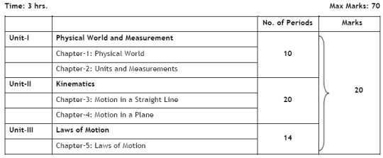
Unit I: Physical World and Measurement 10 Periods

Chapter–1: Physical World Physics-scope and excitement; nature of physical laws; Physics, technology and society. Chapter–2: Units and Measurements Need for measurement: Units of measurement; systems of units; SI units, fundamental and derived units. Length, mass and time measurements; accuracy and precision of measuring instruments; errors in measurement; significant figures. Dimensions of physical quantities, dimensional analysis and its applications.

Unit II: Kinematics 20 Periods

Chapter–3: Motion in a Straight Line Frame of reference, Motion in a straight line: Position-time graph, speed and velocity. Elementary concepts of differentiation and integration for describing motion, uniform and non-uniform motion, average speed and instantaneous velocity, uniformly accelerated motion, velocity - time and position-time graphs. Relations for uniformly accelerated motion (graphical treatment). Chapter–4: Motion in a Plane Scalar and vector quantities; position and displacement vectors, general vectors and their notations; equality of vectors, multiplication of vectors by a real number; addition and subtraction of vectors, relative velocity, Unit vector; resolution of a vector in a plane, rectangular components, Scalar and Vector product of vectors. Motion in a plane, cases of uniform velocity and uniform acceleration-projectile motion, uniform circular motion.

Unit III: Laws of Motion 14 Periods

Chapter–5: Laws of Motion Intuitive concept of force, Inertia, Newton's first law of motion; momentum and Newton's second law of motion; impulse; Newton's third law of motion. Law of conservation of linear momentum and its applications. Equilibrium of concurrent forces, Static and kinetic friction, laws of friction, rolling friction, lubrication. Dynamics of uniform circular motion: Centripetal force, examples of circular motion (vehicle on a level circular road, vehicle on a banked road).

Unit IV: Work, Energy and Power 12 Periods

Chapter–6: Work, Engery and Power Work done by a constant force and a variable force; kinetic energy, work-energy theorem, power. Notion of potential energy, potential energy of a spring, conservative forces: conservation of mechanical energy (kinetic and potential energies); non-conservative forces: motion in a vertical circle; elastic and inelastic collisions in one and two dimensions.

Unit V: Motion of System of Particles and Rigid Body 18 Periods

Chapter–7: System of Particles and Rotational Motion Centre of mass of a two-particle system, momentum conservation and centre of mass motion. Centre of mass of a rigid body; centre of mass of a uniform rod. Moment of a force, torque, angular momentum, law of conservation of angular momentum and its applications. Equilibrium of rigid bodies, rigid body rotation and equations of rotational motion, comparison of linear and rotational motions. Moment of inertia, radius of gyration, values of moments of inertia for simple geometrical objects (no derivation). Statement of parallel and perpendicular axes theorems and their applications.

Unit VI: Gravitation 12 Periods

Chapter–8: Gravitation Kepler's laws of planetary motion, universal law of gravitation. Acceleration due to gravity and its variation with altitude and depth. Gravitational potential energy and gravitational potential, escape velocity, orbital velocity of a satellite, Geo-stationary satellites.

Unit VII: Properties of Bulk Matter 20 Periods

Chapter–9: Mechanical Properties of Solids Elastic behaviour, Stress-strain relationship, Hooke's law, Young's modulus, bulk modulus, shear modulus of rigidity, Poisson's ratio; elastic energy. Chapter–10: Mechanical Properties of Fluids Pressure due to a fluid column; Pascal's law and its applications (hydraulic lift and hydraulic brakes), effect of gravity on fluid pressure. Viscosity, Stokes' law, terminal velocity, streamline and turbulent flow, critical velocity, Bernoulli's theorem and its applications. Surface energy and surface tension, angle of contact, excess of pressure across a curved surface, application of surface tension ideas to drops, bubbles and capillary rise. Chapter–11: Thermal Properties of Matter Heat, temperature, thermal expansion; thermal expansion of solids, liquids and gases, anomalous expansion of water; specific heat capacity; Cp, Cv - calorimetry; change of state - latent heat capacity. Heat transfer-conduction, convection and radiation, thermal conductivity, qualitative ideas of Blackbody radiation, Wein's displacement Law, Stefan's law, Green house effect.

Unit VIII: Thermodynamics 12 Periods

Chapter–12: Thermodynamics Thermal equilibrium and definition of temperature (zeroth law of thermodynamics), heat, work and internal energy. First law of thermodynamics, isothermal and adiabatic processes. Second law of thermodynamics: reversible and irreversible processes, Heat engine and refrigerator.

Unit IX: Behaviour of Perfect Gases and Kinetic Theory of Gases 08 Periods

Chapter–13: Kinetic Theory Equation of state of a perfect gas, work done in compressing a gas. Kinetic theory of gases - assumptions, concept of pressure. Kinetic interpretation of temperature; rms speed of gas molecules; degrees of freedom, law of equi-partition of energy (statement only) and application to specific heat capacities of gases; concept of mean free path, Avogadro's number.

Unit X: Mechanical Waves and Ray Optics 16 Periods

Chapter–14: Oscillations and Waves Periodic motion - time period, frequency, displacement as a function of time, periodic functions. Simple harmonic motion (S.H.M) and its equation; phase; oscillations of a loaded spring-restoring force and force constant; energy in S.H.M. Kinetic and potential energies; simple pendulum derivation of expression for its time period. Free, forced and damped oscillations (qualitative ideas only), resonance. Wave motion: Transverse and longitudinal waves, speed of wave motion, displacement relation for a progressive wave, principle of superposition of waves, reflection of waves, standing waves in strings and organ pipes, fundamental mode and harmonics, Beats, Doppler effect. Chapter–15: RAY OPTICS 18 Periods Ray Optics: Reflection of light, spherical mirrors, mirror formula, refraction of light, total internal reflection and its applications, optical fibres, refraction at spherical surfaces, lenses, thin lens formula, lensmaker's formula, magnification, power of a lens, combination of thin lenses in contact, refraction and dispersion of light through a prism. Scattering of light - blue colour of sky and reddish apprearance of the sun at sunrise and sunset. Optical instruments: Microscopes and astronomical telescopes (reflecting and refracting) and their magnifying powers. The record, to be submitted by the students, at the time of their annual examination, has to include: Record of at least 15 Experiments , to be performed by the students. Record of at least 5 Activities , to be demonstrated by the teachers. Report of the project to be carried out by the students.

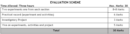
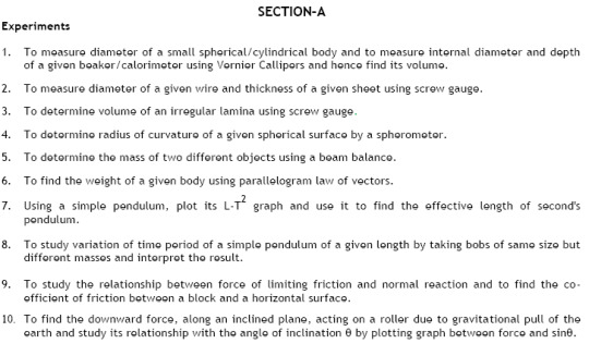
Activities (for the purpose of demonstration only) 1. To make a paper scale of given least count, e.g., 0.2cm, 0.5 cm 2. To determine mass of a given body using a metre scale by principle of moments 3. To plot a graph for a given set of data, with proper choice of scales and error bars 4. To measure the force of limiting friction for rolling of a roller on a horizontal plane 5. To study the variation in range of a projectile with angle of projection 6. To study the conservation of energy of a ball rolling down on an inclined plane (using a double inclined plane) 7. To study dissipation of energy of a simple pendulum by plotting a graph between square of amplitude & time SECTION–B Experiments 1. To determine Young's modulus of elasticity of the material of a given wire. 2. To determine the surface tension of water by capillary rise method 3. To determine the coefficient of viscosity of a given viscous liquid by measuring terminal velocity of a given spherical body 4. To determine specific heat capacity of a given solid by method of mixtures 5. a) To study the relation between frequency and length of a given wire under constant tension using sonometer b) To study the relation between the length of a given wire and tension for constant frequency using sonometer. 6. To find the speed of sound in air at room temperature using a resonance tube by two resonance positions. 7. To find the value of v for different values of u in case of a concave mirror and to find the focal length. 8. To find the focal length of a convex lens by plotting graphs between u and v or between 1/u and 1/v. 9. To determine angle of minimum deviation for a given prism by plotting a graph between angle of incidence and angle of deviation. 10. To determine refractive index of a glass slab using a travelling microscope. Activities (for the purpose of demonstration only) 1. To observe change of state and plot a cooling curve for molten wax. 2. To observe and explain the effect of heating on a bi-metallic strip. 3. To note the change in level of liquid in a container on heating and interpret the observations. 4. To study the effect of detergent on surface tension of water by observing capillary rise. 5. To study the factors affecting the rate of loss of heat of a liquid. 6. To study the effect of load on depression of a suitably clamped metre scale loaded at (i) its end (ii) in the middle. 7. To observe the decrease in presure with increase in velocity of a fluid. 8. To observe refraction and lateral deviation of a beam of light incident obliquely on a glass slab. 9. To study the nature and size of the image formed by a (i) convex lens, (ii) concave mirror, on a screen by using a candle and a screen (for different distances of the candle from the lens/mirror). 10. To obtain a lens combination with the specified focal length by using two lenses from the given set of lenses.

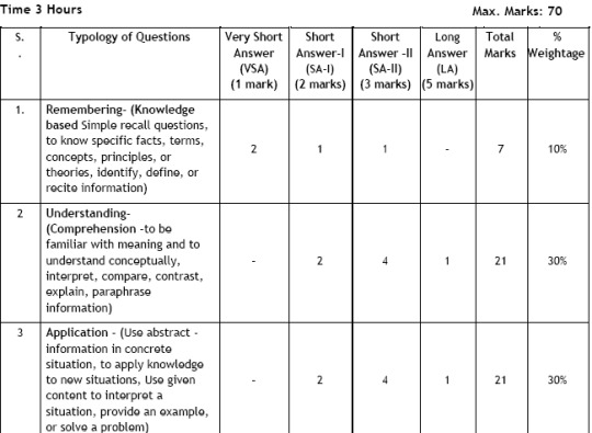
Question Wise Break Up Type of Question Mark per Question Total No. of Questions Total Marks VSA 1 5 05 SA-I 2 7 14 SA-II 3 12 36 LA 5 3 15 Total 27 70 1. Internal Choice: There is no overall choice in the paper. However, there is an internal choice in one question of 2 marks weightage, one question of 3 marks weightage and all the three questions of 5 marks weightage. 2. The above template is only a sample. Suitable internal variations may be made for generating similar templates keeping the overall weightage to different form of questions and typology of questions same. Read the full article