13maxg

[13maxg]

Apache Beam - Cloud computing in banking

[13maxg]

[13maxg]

The formula for Sunflower sequence is following:

$S_n = \sqrt{n}\exp(i \pi (3-\sqrt{5} ) n)$

The animation above shows what happens when $exp$ is replaced with its Padé approximation.  The time represents the polynomial degrees of both numerator and denominator. For non-integer times linear approximation between two nearest integer degrees is performed.

Animation was written in C++ using my library OptimizedGif.

[13maxg]

pdf ,drive,

[13maxg]

[source]

[13maxg]

Diffusion equation with mask

The animations shows evolution of some heatmaps that agrees with the diffusion equation and has some custom boundaries.

My implementation works on discretized torus [0,1]x[0,1] and uses a binary mask that tells where the differences can be applied. The Crank-Nicolson method has been used to solve the equation.

See [source]

[13maxg]

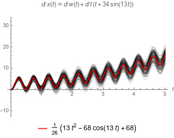
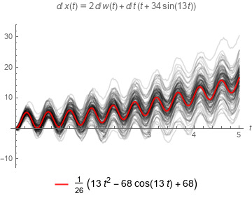
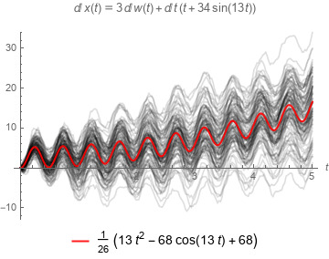
Side effects on tampering with Brownian Motion and stochastic differential equations

Some code can be found here

[13maxg]

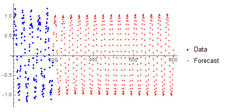
Stochastic motion on a circle

See the system of stochastic differential equations in [PDF].

[13maxg]

Vasicek model calibration

Test on artificial data: time= 0.0833333; market= 0.997561; ours= 0.997474; diff= 8.65876e-05 time= 0.166667; market= 0.995122; ours= 0.994859; diff= 0.00026265 time=     0.25; market= 0.992683; ours= 0.992245; diff= 0.000437884 time=        1; market= 0.970732; ours= 0.974116; diff= 0.0033847 time=        2; market= 0.968293; ours= 0.964037; diff= 0.00425525 time=        3; market= 0.965854; ours= 0.960163; diff= 0.00569088 time=        5; market= 0.960976; ours=  0.95594; diff= 0.00503538 time=        8; market= 0.953659; ours= 0.950497; diff= 0.00316203 time=       21; market= 0.921951; ours= 0.927405; diff= 0.00545383

PDF, GDRIVE, BITBUCKET

[13maxg]

Complex Interval Multiplication

Today I got inspired by Ramon E. Moore‘s “Introduction to Interval Analysis“. I programmed those two images in C++ using my OptimizedGif library and switching FPU rounding mode.

A complex interval is a pair of two intervals, one for real and one for imaginary part. Arithmetic operations are defined intervals, which I extended to complex intervals. Details can be found on my Google Drive.

On the images:

The circle represents the unit circle on complex plane

The red square represents Complex Interval A

The green square represents Complex Interval B

The blue square is result of A * B

See the source here.

[13maxg]

Dropping balls by means of  Golden Angle

Let us have a unit circle located in a 3D space. I want to simulate spawning a balls which center lie on the circle, such that each is generated by some multiplicity of the Golden Angle. I want to spawn one ball at a time and I want a gravity to works on them.

Using blender I made such simulation. Each ball has the same mass and friction parameter. The source code you can find here.

[13maxg]

Dice fairness verification

The image tells how many throws of dice the Chi Squared Test requires to make sure that the test will in no more than 10% of the cases commit error type I  and  in no more than 20% error type II. The horizontal axis represents how much the dice is biased.

See more here.

[13maxg]

Pics I found in my archives

[13maxg]

An application of the rectangular Stoke's theorem

In this paper I want to present how one could apply the rectangular Stoke's theorem to integrate a function $f:\mathbb{R}^N\rightarrow\mathbb{R}$, $N\ge2$, over a rectangular region $\mathcal{R}$. Firstly I will  referee to the theorem. The theorem uses differential forms, so I will show how to construct one from the $f$. Finally I will evaluate the integrals from the theorem and present an example.

[See PDF here]

[13maxg]

Auto regressive model

See more at [PDF]

[13maxg]

The alien integration

AlienPlot3D[f[{u,v}], {u, -1, 1}, {v, -1, 1}]

[See pdf here]

[13maxg]

The co-area formula and Fubini’s theorem

[See pdf here]