andidatachief56

[andidatachief56]

data analysis tool, wk4

Hello,

Question: Is there a correlation between income per person, alcohol consumption and life expectation.

For this a pearsson correlation was programmed between a) alcohol consumption und the life expectancy with income per person as moderator b) income per person and life expectancy with alcohol consumption as moderator

Dataset: gapminder.csv

Program: Since the 3 variables are quantative, 2 categorical sub variables were build for both moderators for minor & high income (incomegrp) and small & high alcohol consumption (alccons).

By using the Pearsson- correlation function of the stats- module the correlation bteween both variables are calculated and displayed using the seaborn.regplot function.

Result:   There is no correlation between alcohol consumption and life expectancy independently of the incoming, but a clear correlation between incomming and life expectancy, rich people life longer (show higher r- values). This is independenly of the alcohol consumption.

Program:

[andidatachief56]

data analysis tools week 3

Hello,

following correlation is to be calculated:   Is there a correlation between the Age und the quantity of beer consuming each day.

Dataset: nesarc_pds.csv

2 quantative Variables choosen: 342-343 S2AQ5D NUMBER OF BEERS USUALLY CONSUMED ON DAYS WHEN DRANK BEER IN LAST 12 MONTHS 18268 1-42. Number of beers    78 99. Unknown    24747 BL. NA did not drink or unknwon

68-69 AGE     AGE       43079 18-97. Age in years      14 98. 98 years or older

Program: A sub- dataframe was created with the 2 choosen variables 'AGE' and 'S2AQ5D'. All unknown and NA rows dropped as well as all drinker of only 1 beer to remove the ground noise. By using the Pearsson- correlation function of the stats- module the correlation between both variables are calculated

Result:   The r- value = -0,15, that means almost no correlation between the Age and the quantity of beer each day.  

------------------------------------------------------------------------------------------------------- Program:

import os import pandas import numpy import seaborn import scipy.stats

# define individual name of dataset data = pandas.read_csv('nesarc_pds.csv', low_memory=False)

# recode missing values to python missing (NaN) data['S2AQ5D']=data['S2AQ5D'].replace('99', numpy.nan)    # defined as char data['S2AQ5D']=data['S2AQ5D'].replace(' ', numpy.nan)    # needed before set to numeric

# new code setting variables you will be working with to numeric data['S2AQ5D'] = pandas.to_numeric(data['S2AQ5D'], errors='coerce')

# data subset only for needed columns sub1 = data[['AGE','S2AQ5D']]

#make a copy of my new subsetted data   !! wichtig !!!   Remove NaN sub2 = sub1.copy()

print(len(sub2))              # No. of rows print(len(sub2.columns))  

sub2 = sub2.dropna()

print(' ---  nach dropNA ----') print(len(sub2))              # No. of rows print(len(sub2.columns))   print(sub2.value_counts(subset='S2AQ5D', normalize=True))    # in Prozent

sub2=sub2[(sub2['S2AQ5D']>1)]      # drop all rows with 1 beer

print(' ---  nach remove 1-3 ----') print(len(sub2))              # No. of rows print(len(sub2.columns))   print(sub2.value_counts(subset='S2AQ5D', normalize=True))    # in Prozent

scat1 = seaborn.regplot(x="AGE", y="S2AQ5D", fit_reg=True, data=sub2) plt.xlabel('AGE') plt.ylabel('Drinking beer per day') plt.title('Scatterplot for the Association Between AGE and consuming beer')

print ('association between AGE and consuming beer') print (scipy.stats.pearsonr(sub2['AGE'], sub2['S2AQ5D']))

---------------------------------------------------------------------------------------------

association between AGE and consuming beer (-0.15448800873680543, 1.7107443117251883e-60)

[andidatachief56]

Wk02  CHI square test

Hello,

the H0- hypothesis is, that there is no difference in drinking behaviour between the regions in US.

Dataset: nesarc_pds.csv

Categorical Variables:   1.  337-337 S2AQ5A DRANK ANY BEER IN LAST 12 MONTHS    18346 1. Yes   8562 2. No    38 9. Unknown     16147 BL. NA, former drinker or lifetime abstainer 2.  41-41 REGION CENSUS REGION    8209 1. Northeast   8991 2. Midwest   16156 3. South    9737 4. West

Program: A crosstable was generated by panda.crosstab- fuction with 2 categoric variables 'S2AQ5A' and 'Region'. The CHI- square and p- value was calculated by scipy.stats.chi2 - function for all regions and 3 post-hoc tests with 2 by 2 - comparsions.  

Result:   The H0- hypothesis has to be rejected (p<<0,05) for comparing all regions and for 2 post-hoc tests. Only for the post-hoc comparision between West amd Midwest the H0 can be acctepted (P>0,05).

------------------------------------------------------------------------------------------------------- Program:

import os import pandas import numpy import scipy.stats

# define individual name of dataset data = pandas.read_csv('nesarc_pds.csv', low_memory=False)

# 2x categorical Variables used in program # 337-337 S2AQ5A DRANK ANY BEER IN LAST 12 MONTHS # 18346 1. Yes   8562 2. No    38 9. Unknown     16147 BL. NA, former drinker or lifetime abstainer

# 41-41 REGION CENSUS REGION # 8209 1. Northeast   8991 2. Midwest   16156 3. South    9737 4. West

# recode missing values to python missing (NaN) data['S2AQ5A']=data['S2AQ5A'].replace('9', numpy.nan)    # defined as char data['S2AQ5A']=data['S2AQ5A'].replace(' ', numpy.nan)    # needed before set to numeric

# new code setting variables you will be working with to numeric data['S2AQ5A'] = pandas.to_numeric(data['S2AQ5A'], errors='coerce')

# data subset only for needed columns sub1 = data[['REGION','S2AQ5A']]

#make a copy of my new subsetted data     Remove NaN sub2 = sub1.copy() sub2 = sub2.dropna()

recode2 = {1: "Northeast", 2: "Midwest", 3: "South", 4: "West"} sub2['REGION']= sub2['REGION'].map(recode2)

print(len(sub2))              # No. of rows print(len(sub2.columns))   print(sub2.head(5))

# contingency (Häufigkeits)- table of observed counts for both variables ct1=pandas.crosstab(sub2['S2AQ5A'], sub2['REGION']) print('----- Cross table  -------') print (ct1)

# column percentages colsum=ct1.sum(axis=0) colpct=ct1/colsum print('----- in %  -------') print(colpct)

# chi-square print () print ('chi-square value, p value, df, expected counts') cs1= scipy.stats.chi2_contingency(ct1) print (cs1)

print () print ('....... Post Hoc  Compare 1  NW - MW  .........') recode3 = {"Northeast": "Northeast", "Midwest": "Midwest" } sub2['COMP1']= sub2['REGION'].map(recode3)

# contingency table of observed counts ct2=pandas.crosstab(sub2['S2AQ5A'], sub2['COMP1']) print (ct2)

# column percentages colsum=ct2.sum(axis=0) colpct=ct2/colsum print(colpct)

print ('chi-square value, p value, df, expected counts') cs2= scipy.stats.chi2_contingency(ct2) print (cs2)

print () print ('....... Post Hoc  Compare 2  W - MW  .........') recode3 = {"West": "West", "Midwest": "Midwest" } sub2['COMP2']= sub2['REGION'].map(recode3)

# contingency table of observed counts ct2=pandas.crosstab(sub2['S2AQ5A'], sub2['COMP2']) print (ct2)

# column percentages colsum=ct2.sum(axis=0) colpct=ct2/colsum print(colpct)

print ('chi-square value, p value, df, expected counts') cs2= scipy.stats.chi2_contingency(ct2) print (cs2)

print () print ('....... Post Hoc  Compare 3  W - S  .........') recode3 = {"West": "West", "South": "South" } sub2['COMP3']= sub2['REGION'].map(recode3)

# contingency table of observed counts ct2=pandas.crosstab(sub2['S2AQ5A'], sub2['COMP3']) print (ct2)

# column percentages colsum=ct2.sum(axis=0) colpct=ct2/colsum print(colpct)

print ('chi-square value, p value, df, expected counts') cs2= scipy.stats.chi2_contingency(ct2) print (cs2)

------------------------------------------------------------------------------- Output: ------------------------------------------------------------------------------

----- Cross table  ------- REGION  Midwest  Northeast  South  West S2AQ5A                                 1.0        4271       3535   6043  4497 2.0        1811       1953   2951  1847 ----- in %  ------- REGION   Midwest  Northeast     South      West S2AQ5A                                         1.0     0.702236   0.644133  0.671892  0.708859 2.0     0.297764   0.355867  0.328108  0.291141

chi-square value, p value, df, expected counts (73.07946685879071, 9.346703898504186e-16, 3, array([[4146.7359893 , 3741.74401665, 6132.1511818 , 4325.36881225],       [1935.2640107 , 1746.25598335, 2861.8488182 , 2018.63118775]]))   -->  H0- hypotheses rejected:  p= 9,3e-16  significant more drinker in Midwest & West than Northeast & South

....... Post Hoc  Compare 1  Northeast - Midwest  ......................................... COMP1   Midwest  Northeast S2AQ5A                     1.0        4271       3535 2.0        1811       1953 COMP1    Midwest  Northeast S2AQ5A                     1.0     0.702236   0.644133 2.0     0.297764   0.355867 chi-square value, p value, df, expected counts (44.10875595370776, 3.106283333437607e-11, 1, array([[4103.37873812, 3702.62126188],       [1978.62126188, 1785.37873812]]))

-->  H0- hypotheses rejected:  p= 3,1e-11  significant more drinker in Midwest than Northeast     ....... Post Hoc  Compare 2  West - Midwest  ........................................ COMP2   Midwest  West S2AQ5A               1.0        4271  4497 2.0        1811  1847 COMP2    Midwest      West S2AQ5A                     1.0     0.702236  0.708859 2.0     0.297764  0.291141 chi-square value, p value, df, expected counts (0.6241389726531966, 0.4295133634241102, 1, array([[4291.56413971, 4476.43586029],       [1790.43586029, 1867.56413971]]))   H0- hypotheses confirmed:  p= 0,42  no difference in drinking behaviour between West and Midwest   ....... Post Hoc  Compare 3  West - South  .......................................... COMP3   South  West S2AQ5A             1.0      6043  4497 2.0      2951  1847 COMP3      South      West S2AQ5A                     1.0     0.671892  0.708859 2.0     0.328108  0.291141 chi-square value, p value, df, expected counts (23.476544240410604, 1.2644599462751704e-06, 1, array([[6180.51636458, 4359.48363542],       [2813.48363542, 1984.51636458]]))  

[andidatachief56]

Data analysis tools wk01

Task:  The hypothesis is to be verified that there is a significant relation between the number of beers drink per year and the region living in USA.  

Dataset used:  Nesarc_pds.csv

Explanation : The variables used are:  'S2AQ5B'  -  frequency of beer drinking 'S2AQ5D'  - No of beers each days. Secondary variables was calculated to ‘Beernum’ - No of beers per year, used as Quantitative variable in the .ols  - function. As categorical the variable ‘Region’ was used.  F- Statistic and p- value was calculated with the .ols- function in overall. A comparison post hoc test calculated the relation.

Program:

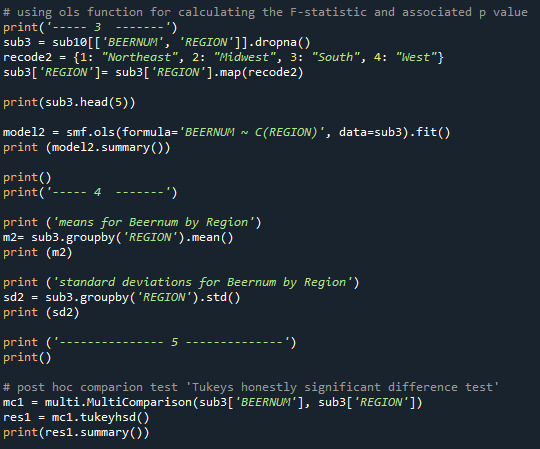
Conclusion: With the ols- function no relation between No. of beers drinking per beer and the region is shown, the null hypothesis has to be rejected. The p- value is 0,000784, so by far < 0,05.

The mean values for beers per year is between 285 for people living in Midwest and 224 beers in Northeast.

The post hoc comparison calculate now a signicant relation between Midwest/ Northeast, Midwest/West and South/Notheast, here the mean values has the greatest difference, the null hypothesis is accepted for those Regions.

[andidatachief56]

week 4 assignment

Course: Data management and visualization Assignment:  wk4 Dataset: Nesarc

3 selected Variables from nesarc- dataset has been used for the graphs: - ‘AGEGR’:  Age groups built from variable ‘AGE’ for young (17-30y), mid-age (30-60) and old (60-90) persons showing the age. Defined as categorical. AGE is numeric. - ‘S3AQ3C1′: Usual quantity if cigarettes, defined as numeric. - ‘TAB12MDX’: Nicotine dependence, variables redefined as numeric.

Program:

Result:  Follwowing graphs has been generated: 

1. Univariable graph showing showing the number of persons (frequency distribution) per AGE smoking in the last 12 months. The variable AGR is grouped in 3 groups.  Result: Most of the smokers coming from mid-age group with ages between 30 and 60.

2. Bi- variable graph showing of nicotine dependent (Var: ‘TAB12MDX’ - shown in proportion) persons in relation to the number of cigrarettes smoking each day (Var:  ‘S3AQ3C1′). Result:  The more cigarettes smoked each day the higher the proportion of nicotine dependency, no big surprise.

3. Bi- variable Scatterplot of ‘AGE’ (x-axis) in relation to quantity of smoking (y-axis). Result:  No dependency visible between the age and the quantity of smoking, high frequency smoker are visible in younger and older age.

[andidatachief56]

week 3 assigment

Course: Data management and visualization Assigment week 3 Dataset:  nesarc.csv

Research: - How many drinker and smoker did both in the last 12 months, drinking AND smoking. - Which AGE group in relation mostly involved in drinking AND smoking.

Program: From the dataset nesarc.csv a subgroup was defined with the variables CHECK321, S2AQ3 and AGE. The subgroup was filtered to those observations who drink or smoke and a secondary variable created with the value ‘2′ for those who drink AND smoke both in the last 12 months and the frequency calculated.

Next the persons were grouped by CUT- function into young (17-30 year old), midage (30-60) and old (60-90) persons and the frequency of drinker and smoker evaluated.

Result: - Almost the half (49,5%) of drinkers and smokers did both, drinking and smoking, in the last 12 months. - In related to all interviewed people the young- and mid- group have the same rate of drinker & smoker (21,5%), whereas the old group have less rate (11%).

Program:

Output:

[andidatachief56]

Hello,

2 sub_groups were built for male and female (Variable: SEX) who smoked in the pasted 12 months (CHECK321).

Frequency distributions was done for each sub group on nicotine dependency and age.

Output:  Nicotine dependancy slightly higher for male smoker (54,9%) than for female (50,2%). And, male smoker are older than female.

Programming Code:

# Import libraries (packages) import pandas import numpy

# define individual name of dataset data = pandas.read_csv('nesarc_pds.csv', low_memory=False)

# upper-case all DataFrame column names- place after code for loading data above data.columns = list(map(str.upper, data.columns))

# bug fix for display formats to avoid run time errors - put after code for loading data above pandas.set_option('display.float_format', lambda x: '%f' % x)

print(len(data))  # number of observations (rows) print(len(data.columns))  # number of variables (columns)

# checking the format of your variables data['ETHRACE2A'].dtype

# setting variables you will be working with to numeric data['TAB12MDX'] = pandas.to_numeric(data['TAB12MDX']) data['CHECK321'] = pandas.to_numeric(data['CHECK321']) data['S3AQ3B1'] = pandas.to_numeric(data['S3AQ3B1']) data['SEX'] = pandas.to_numeric(data['SEX']) data['AGE'] = pandas.to_numeric(data['AGE'])

print("counts 1 -male, 2- female") c1 = data['SEX'].value_counts(sort=False, dropna=False) print(c1)

print("percentages") p1 = data['SEX'].value_counts(sort=False, normalize=True) * 100 print(p1) print()

# create sub group for male and female and smoked in the past 12 months sub_male = data[(data['SEX'] == 1) & (data['CHECK321']==1)] sub_female = data[(data['SEX'] == 2) & (data['CHECK321']==1)]

print("Nicotine dependence 0-No  1-yes for male smoked past 12 months") c2 = sub_male['TAB12MDX'].value_counts(sort=False) print(c2)

p2 = sub_male['TAB12MDX'].value_counts(sort=False, normalize=True) * 100 print(p2,'in %') print()

print("Nicotine dependence 0-No  1-yes for female smoked past 12 months") c3 = sub_female['TAB12MDX'].value_counts(sort=False) print(c3)

p3 = sub_female['TAB12MDX'].value_counts(sort=False, normalize=True) * 100 print(p3,'in %') print()

print('count male - AGE in percentage') p4 = sub_male['AGE'].value_counts(sort=True, normalize=True) * 100 print(p4) print()

print('count femal Age in percentage') p5 = sub_female['AGE'].value_counts(sort=True, normalize=True) * 100 print(p5)

Output:

counts 1 -male, 2- female 1    18518 2    24575 Name: SEX, dtype: int64 percentages 1   42.972176 2   57.027824 Name: SEX, dtype: float64

Nicotine dependence 0-No  1-yes for male smoked past 12 months 0    2659 1    2184 Name: TAB12MDX, dtype: int64 0   54.903985 1   45.096015 Name: TAB12MDX, dtype: float64 in %

Nicotine dependence 0-No  1-yes for female smoked past 12 months 1    2547 0    2523 Name: TAB12MDX, dtype: int64 1   50.236686 0   49.763314 Name: TAB12MDX, dtype: float64 in %

count male smoker  - Age in percentage 47   2.787528 45   2.787528 40   2.766880 42   2.560396 38   2.560396 Name: AGE, Length: 72, dtype: float64

count femal smoker - Age in percentage 37   3.136095 40   2.761341 38   2.682446 24   2.682446 30   2.623274 Name: AGE, Length: 76, dtype: float64

[andidatachief56]

Relation lifeexpectancy to income

Hello together,

in terms of the 'data managment and visualization'- course I have decided to choose the following data assigment.

Step 1:  Choose data set: The variables ‘incomeperperson’ and ‘lifeexpectancy’ have been selected from the dataset ‘gapminder.csv’.  The data set provides a mean value for both variables for each country wordwide.

Step 2: Research question and hypothesis: The question for research is whether there is a dependancy between the life expectancy to the salary (income) of a person. Hypothesis is that with higher salary the life expectancy would also increase.

Step 3: Literature review: Literature review was done on the document “Income distribution and life expectancy “ by R G Wilkonson, see link. https://www.ncbi.nlm.nih.gov/pmc/articles/PMC1881178/pdf/bmj00056-0043.pdf

The relation between average income and life expectancy was assessed using figures of gross national product per head  for 23 countries in the Organisation for Economic Cooperation and Development.'

Step 4: References used for literature review Several (>30) references are mentioned:

.......

Step 5: Summary of findings The correlation between the increases in gross national product per head and in life expectancy over the 16 years 1970-1 to 1986-7 was almost non-existent at 0 07. These data seem to confirm that there is, at best, only a weak relation between gross national product per head and life expectancy in developed countries.

[andidatachief56]

First Assignement

Hier Text

[andidatachief56]

data zum quadrat