arpitabathija

[arpitabathija]

Data Visualization week 4 Assignment

Univariate graphs are shown on top for categorical created variable (diameter of circle in 4 categories) and quantitative variable (diameter of circle of mars crater). We see that maximum number of craters fall in the smallest diameter bin.

Next is a scatter plot between diameter and depth of the craters. We do see a positive relation that is as diameter increase depth also increases.

Next we plot a bivariate bar graph between number of layers and depth. we do see that number of layers is largest for the deepest craters.

[arpitabathija]

Making Data Management Decisions

First did the data cleaning by removing missing and unknown data. Then created ethnicity variable:

3 Being White which is the majority

4 Being Black/African

2 Being Hispanic

6 Being Asian

5 Being Native American in minority

[arpitabathija]

Data management and visualization Assignment week2

[arpitabathija]

Data Management Lesson 1

Gap Minder Dataset

Research Question: Is Life expectancy related to whether a person is from a developed country

The second variable can be income. Is Life expectancy dependent on income?

[arpitabathija]

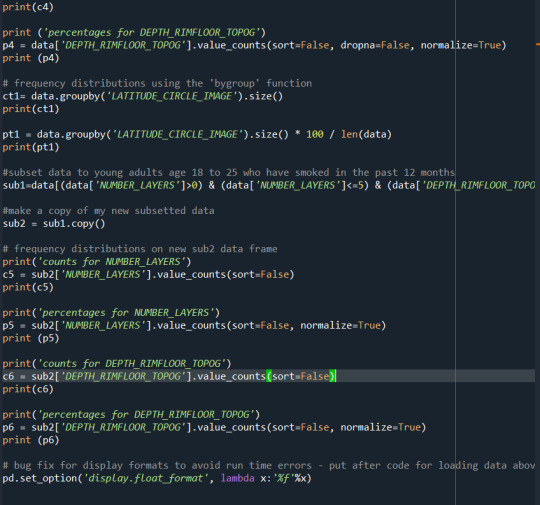
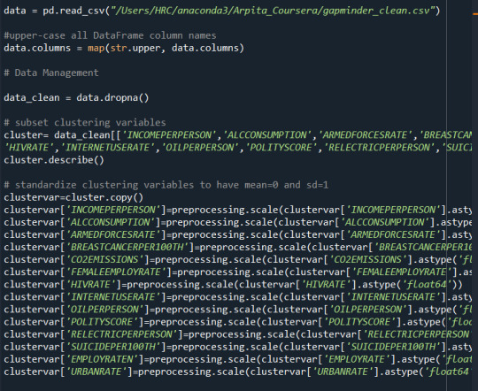
Assignment 4

A k-means cluster analysis was conducted to identify underlying subgroups of lifestyles/habits based on 14 variables. Clustering variables included quantitative variables measuring

INCOME PER PERSON, ALC CONSUMPTION, ARMED FORCES RATE, BREAST CANCER PER 100TH. CO2 EMISSIONS, FEMALE EMPLOYRATE, HIV RATE, INTERNET USE RATE, OIL PER PERSON, POLITY SCORE, ELECTRIC PER PERSON, SUICIDE PER 100TH, EMPLOY RATE, URBAN RATE

All clustering variables were standardized to have a mean of 0 and a standard deviation of 1.

Data were randomly split into a training set that included 70% of the observations (N=39) and a test set that included 30% of the observations (N=17). A series of k-means cluster analyses were conducted on the training data specifying k=1-9 clusters, using Euclidean distance. The variance in the clustering variables that was accounted for by the clusters (r-square) was plotted for each of the nine cluster solutions in an elbow curve to provide guidance for choosing the number of clusters to interpret.

Figure 1. Elbow curve of r-square values for the nine cluster solutions

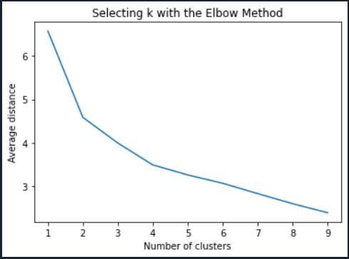
The elbow curve was inconclusive, suggesting that the 2 and 4 cluster solutions might be interpreted. The results below are for an interpretation of the 4-cluster solution.

Canonical discriminant analyses was used to reduce the 14 clustering variable down a few variables that accounted for most of the variance in the clustering variables. A scatterplot of the first two canonical variables by cluster (Figure 2 shown below) indicated that the observations in clusters 1 through 4 were distinct and did not overlap with the other clusters. Observations in cluster 4 or deep red were spread out more than the other clusters, showing high within cluster variance.

Figure 2. Plot of the first two canonical variables for the clustering variables by cluster.

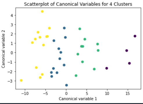
The means on the clustering variables showed that, compared to the other clusters, cluster 1 had highest HIV Rate and cluster 4 had the income per person, highest urban rate, employ rate, oil per person, electric per person and internet use rate. All in all cluster 4 had a better life and thus higher life expectancy was evident. And higher HIV RATE points to lower life expectancy.

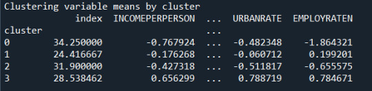
In order to externally validate the clusters, an Analysis of Variance (ANOVA) was conducting to test for significant differences between the clusters on LIFE EXPECTANCY. A tukey test was used for post hoc comparisons between the clusters. The tukey post hoc comparisons showed significant differences between clusters on, LIFE EXPECTANCY with the exception that clusters 2 and 3 were not significantly different from each other. People in cluster 4 had the highest LIFE EXPECTANCY (mean=78.06, sd=4.6), and cluster 1 had the lowest LIFE EXPECTANCY (mean=68.25, sd=10.31).

[arpitabathija]

Assignment 3

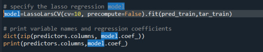
A lasso regression analysis was conducted to identify a subset of variables from a pool of 14 quantitative predictor variables that best predicted a quantitative response variable measuring life expectancy across different countries.

Of the 14 predictor variables, 6 were retained in the selected model. During the estimation process, HIV rate was most strongly negatively associated with life expectancy. Internet use, income per person were next positively associated with life expectancy. Other predictors associated were urban rate, suicide rate and polity score.

The code and output is given below.

[arpitabathija]

Assignment 2 Random Forest

Number of layers is the target variable on Mars crater data. Depth of rim of floor is the most important exploratory variable with 0.3355 and next is diameter of the crater 0.26. 1 or 2 trees is enough and 25 is too many for random forest.

[arpitabathija]

Assignment 1 Decision Tree

2264 experimented with smoking and 481 didnot. Further categorized by bio-sex and it turned out it varied by just a 104 from the smokers. So sex is not a very important variable for experimentalists with smoking