captaindentex

[captaindentex]

A model to predict rainfall from meteorological variables

Introduction to the Research Question

The purpose of this study was to identify possible predictors of Rainfall in Australia from multiple meteorological related factors such as Temperature, Humidity, Pressure etc. 

As a water resources engineer, my scientific interest is to predict future rainfall and be able to design flood control and water management projects. At present I can only rely on past recorded rainfall data to predict future rainfall but being able to have a model that predicts rainfall from other meteorological factors is extremely useful when recorded rainfall data are not available.  

Methods

Research was based on meteorological data from the Bureau of Meteorology of the Australian Government. The sample includes N=3.223 daily records of various weather observations recorded at Sydney meteorological station (Copyright Commonwealth of Australia 2010, Bureau of Meteorology) during the period (2007-2018). More analytically the variables used for this research are:

Predictors which include:

a)      Class A pan evaporation (mm) in the 24 hours to 9am

b)      The number of hours of bright sunshine in the day

c)      Humidity (percent) at 9am

d)      Humidity (percent) at 3pm

e)      Atmospheric pressure (hpa) reduced to mean sea level at 9am

f)       Atmospheric pressure (hpa) reduced to mean sea level at 3pm

g)      Temperature (degrees C) at 9am

h)      Temperature (degrees C) at 3pm

The response variable:

i)       The amount of rainfall recorded for the day in mm

 At Table 1 descriptive statistics of each variable is presented. We can easily assume that there five major prediction factors (Evaporation, Sunshine, Humidity, Pressure and Temperature). Evaporation and Sunshine are recorded once a day while each of the rest is recorded two times a day (9 am and 3 pm) making a total of 8 prediction factors. Looking at the Average column we can make an early assumption that Temperature is in general higher in the afternoon than in the morning whereas the opposite happens for Humidity and Pressure.  

   Variable

N

Average

StDev

Min

Max

Rainfall

3.223

2,85

7,94

0,00

94,40

Evaporation

3.223

5,18

2,78

0,00

18,40

Sunshine

3.223

7,22

3,80

0,00

13,60

Humidity 9am

3.223

68,06

15,03

19,00

100,00

Humidity 3pm

3.223

54,49

16,19

10,00

99,00

Pressure 9am

3.223

1018,36

7,01

986,70

1039,00

Pressure 3pm

3.223

1016,02

7,02

989,80

1036,70

Temp 9am

3.223

17,85

4,91

6,40

36,50

Temp 3pm

3.223

21,58

4,30

10,20

44,70

Table 1. Descriptive Statistics for Data Analytic Variables

 Analysis

Since all our variables are quantitative we perform the Pearson Correlation to examine if there is relationship among them. Analysis shows that there is a modest correlation between Rainfall and Sunshine and Rainfall and Humidity (9am and 3pm). Pearson correlations (Table 2) are approximately 0,30 for those three correlations. Humidity shows a positive correlation which means that greater humidity results to greater rainfall while greater sunshine means lower rainfall something that is in agreement with common sense. The rest of the predictor variables show weak correlation with correlation factors less than 0,15 and even zero in the case of Pressure 9am – Rainfall correlation. Temperature also shows weak correlation and seems to be a non significant prediction factor.

Correlation

Pearson  Correlation factor (r)

Intercept  (p)

Evaporation - Rainfall

-0,13

7,87e-14

Sunshine - Rainfall

-0,31

4,83e-71

Humidity9am - Rainfall

0,33

7,90e-85

Humidity3pm - Rainfall

0,30

1,88e-68

Pressure9am - Rainfall

0,00

0,96e0

Pressure3pm - Rainfall

0,04

0,02e0

Temp9am - Rainfall

-0,05

0,00e0

Temp3pm - Rainfall

-0,14

4,12e-15

Table 2. Pearson Correlation Factors

From the scatterplots (Figure 1) we can see clearly the linear connection between Humidity and Rainfall. Low evaporation seems to happen in low rainfall but the relation is weak and many outliers are presented in the graph. There is also a weak negative connection between Temp 3pm and Rainfall which shows higher afternoon rainfall at low temperatures. Rainfall seems to be independent from pressure since events show a uniform distribution to pressure values.

Figure 1 Association between predictors and Rainfall

Lasso regression with the least angle regression selection algorithm was used to identify the subset of variables that best predicted manufacturing lead time. Lasso regression was selected since the relationship between predictors and response variable is linear and there is a large number of predictors. The least angle regression model starts with no predictors in the model and adds a predictor at each step. It first adds a predictor that is most correlated with the response variable and moves it towards least score estimate until there is another predictor. This is equally correlated with the model residual. It adds this predictor to the model and starts the least square estimation process over again with both variables. The algorithm continues with this process until it has tested all the predictors. Parameter estimates at any step are shrunk and predictors with coefficients that have shrunk to zero are removed from the model and the process starts all over again. The lasso regression model was estimated on a training data set consisting of a random sample of 70% of the batches (N=2.256), and a test data set included the other 30% of the batches (N=967). All predictor variables were standardized to have a mean=0 and standard deviation=1 prior to conducting the lasso regression analysis. Cross validation was performed using k-fold cross validation specifying 10 folds. The change in the cross validation mean squared error rate at each step was used to identify the best subset of predictor variables. Predictive accuracy was assessed by determining the mean squared error rate of the training data prediction algorithm when applied to observations in the test data set.

Lasso regression showed that 7 out of 8 predictors were retained in the selection model. Only the Temp 9am was excluded. Regression coefficients, shown in Table 2, show that Pressure 9am is the variable with the strongest regression coefficient with Pressure 3pm in the second place which means that pressure is most strongly associated with rainfall.

Variable

Regression  Coefficient

Evaporation

-0,38

Sunshine

-0,54

Humidity 9am

1,88

Humidity 3pm

0,71

Pressure 9am

-4.63

Pressure 3pm

3.84

Temp 9am

0.00

Temp 3pm

-0.42

Table 2. Regression Coefficients

Humidity (9am and 3pm) is at the third and fourth place respectively while sunshine comes next. Evaporation and temperature are the least associated variables. The progression of regression coefficients through the model selection process is shown on Figure 2.  

Figure 2. Regression Coefficients Progression.

 The plot shows the relative importance of the predictor selected at any step of the selection process and how the regression coefficients changed with the addition of a new predictor at each step. Similarly, on Figure 3 the change in mean square error is shown. Variability is observed across the individual cross-validation folds in the training dataset but the change in the mean squared error as variables are added to the model follows the same pattern for each fold. It decreases slightly and then levels off to a point at which adding more predictors doesn’t lead to much reduction in the mean squared error. The average mean squared error also follows the same pattern.  

 Figure 3. Mean Squared Error

  The mean squared error (MSE) for the test data (MSE=62.98) differs enough from the MSE for the training data (MSE=48.11), which suggests that predictive accuracy is not stable across the two datasets.  The r-squared values were 0,17 and 0,16 respectively indicating that the selected model explained 17% and 16%  of the variance in rainfall for the training and test sets.

[captaindentex]

Machine Learning for Data Analysis: Assignement 4

#Loading Libraries import numpy as np import pandas as pd import matplotlib import matplotlib.pyplot as plt import scipy.stats as sp import datetime as dt import time as tm import os import csv import seaborn import pydotplus import sklearn.metrics import statsmodels.api as sm import statsmodels.formula.api as smf import statsmodels.stats.multicomp as multi from pandas import Series, DataFrame from io import StringIO from IPython.display import Image from scipy.spatial.distance import cdist from sklearn import tree from sklearn import datasets from sklearn import preprocessing from sklearn.model_selection import train_test_split from sklearn.tree import DecisionTreeClassifier from sklearn.metrics import classification_report from sklearn.metrics import mean_squared_error from sklearn.ensemble import ExtraTreesClassifier from sklearn.ensemble import RandomForestClassifier from sklearn.linear_model import LassoLarsCV from sklearn.cluster import KMeans from sklearn.decomposition import PCA

print('') print('Data File') print('-------------------------------------') file='datamal.csv' data=pd.read_csv(file,low_memory=False) #data.columns=map(str.upper,data.columns) pd.set_option('display.float_format',lambda x: '%f' %x) data['Water']=data['Water'].apply(pd.to_numeric, errors='coerce') #Explanatory variable data['Sanitation']=data['Sanitation'].apply(pd.to_numeric, errors='coerce') #Explanatory variable data['Malaria']=data['Malaria'].apply(pd.to_numeric, errors='coerce') #Response variable

#Remove missing values subdata=data[['Country', 'Water', 'Sanitation', 'Malaria']].dropna()

#Grouping variables subdata['Malgroup']=pd.cut(subdata.Malaria, [0.00, 10000.00, 12000000.00],labels=[0,1])

#Remove missing values sub1=subdata[['Water','Sanitation','Malgroup']].dropna() print('sub1.dtypes\n',sub1.dtypes) print('sub1.describe\n',sub1.describe())

print('') print('# Data Management') print('-------------------------------------') #Split into training and testing sets cluster=sub1[['Water','Sanitation','Malgroup']] print(cluster.describe())

# standardize predictors to have mean=0 and sd=1 clustervar=cluster.copy() clustervar['Water']=preprocessing.scale(clustervar['Water'].astype('float64')) clustervar['Sanitation']=preprocessing.scale(clustervar['Sanitation'].astype('float64')) clustervar['Malgroup']=preprocessing.scale(clustervar['Malgroup'].astype('float64'))

# split data into train and test sets clus_train, clus_test=train_test_split(clustervar, test_size=0.3, random_state=123)

# k-means cluster analysis for 1-9 clusters                                                           clusters=range(1,10) meandist=[]

for k in clusters:    model=KMeans(n_clusters=k)    model.fit(clus_train)    clusassign=model.predict(clus_train)    meandist.append(sum(np.min(cdist(clus_train, model.cluster_centers_, 'euclidean'), axis=1))    / clus_train.shape[0])

print('Plot average distance from observations from the cluster centroid to use the Elbow Method to identify number of clusters to choose')

plt.plot(clusters, meandist) plt.xlabel('Number of clusters') plt.ylabel('Average distance') plt.title('Selecting k with the Elbow Method') plt.show()

# Interpret 3 cluster solution model3=KMeans(n_clusters=3) model3.fit(clus_train) clusassign=model3.predict(clus_train) # plot clusters

pca_2=PCA(2) plot_columns=pca_2.fit_transform(clus_train) plt.scatter(x=plot_columns[:,0], y=plot_columns[:,1], c=model3.labels_,) plt.xlabel('Canonical variable 1') plt.ylabel('Canonical variable 2') plt.title('Scatterplot of Canonical Variables for 3 Clusters') plt.show()

print('BEGIN multiple steps to merge cluster assignment with clustering variables to examine cluster variable means by cluster')

# create a unique identifier variable from the index for the # cluster training data to merge with the cluster assignment variable clus_train.reset_index(level=0, inplace=True) # create a list that has the new index variable cluslist=list(clus_train['index']) # create a list of cluster assignments labels=list(model3.labels_) # combine index variable list with cluster assignment list into a dictionary newlist=dict(zip(cluslist, labels)) newlist # convert newlist dictionary to a dataframe newclus=DataFrame.from_dict(newlist, orient='index') newclus # rename the cluster assignment column newclus.columns = ['cluster']

# now do the same for the cluster assignment variable # create a unique identifier variable from the index for the # cluster assignment dataframe # to merge with cluster training data newclus.reset_index(level=0, inplace=True) # merge the cluster assignment dataframe with the cluster training variable dataframe # by the index variable merged_train=pd.merge(clus_train, newclus, on='index') merged_train.head(n=100) # cluster frequencies merged_train.cluster.value_counts()

print('END multiple steps to merge cluster assignment with clustering variables to examine cluster variable means by cluster') # FINALLY calculate clustering variable means by cluster clustergrp=merged_train.groupby('cluster').mean() print ("Clustering variable means by cluster") print(clustergrp)

A k-means cluster analysis was conducted to identify countries with Malaria cases based on their Water and Sanitation Access. . All clustering variables were standardized to have a mean of 0 and a standard deviation of 1.

Data were randomly split into a training set that included 70% of the observations (N=62) and a test set that included 30% of the observations (N=26). A series of k-means cluster analyses were conducted on the training data specifying k=1-9 clusters, using Euclidean distance. The variance in the clustering variables that was accounted for by the clusters (r-square) was plotted for each of the nine cluster solutions in an elbow curve to provide guidance for choosing the number of clusters to interpret.  

The elbow curve was inconclusive, suggesting that the 3 and 5-cluster solutions might be interpreted. The results below are for an interpretation of the 3-cluster solution.  The scatter plot shows no densely packed clusters which menas low correlation

The means on the clustering variables showed that, compared to the other clusters, countries in cluster 0 have moderate Water and Sanitation Access and Malaria Cases. Countries in cluster 1 had the lowest Water and Sanitation Access while Malaria Caases is moderates. Countries in cluster 2 have the lowest Malaria Cases with moderate Water and Sanitation Access

[captaindentex]

Machine Learning for Data Analysis: Assignement 3

#Loading Libraries import numpy as np import pandas as pd import matplotlib import matplotlib.pyplot as plt import scipy.stats as sp import datetime as dt import time as tm import os import csv import seaborn import pydotplus import sklearn.metrics import statsmodels.api as sm import statsmodels.formula.api as smf import statsmodels.stats.multicomp as multi from pandas import Series, DataFrame from io import StringIO from IPython.display import Image from scipy.spatial.distance import cdist from sklearn import tree from sklearn import datasets from sklearn import preprocessing from sklearn.model_selection import train_test_split from sklearn.tree import DecisionTreeClassifier from sklearn.metrics import classification_report from sklearn.metrics import mean_squared_error from sklearn.ensemble import ExtraTreesClassifier from sklearn.ensemble import RandomForestClassifier from sklearn.linear_model import LassoLarsCV from sklearn.cluster import KMeans from sklearn.decomposition import PCA

print('') print('Data File') print('-------------------------------------') file='datamal.csv' data=pd.read_csv(file,low_memory=False) #data.columns=map(str.upper,data.columns) pd.set_option('display.float_format',lambda x: '%f' %x) data['Water']=data['Water'].apply(pd.to_numeric, errors='coerce') #Explanatory variable data['Sanitation']=data['Sanitation'].apply(pd.to_numeric, errors='coerce') #Explanatory variable data['Malaria']=data['Malaria'].apply(pd.to_numeric, errors='coerce') #Response variable

#Remove missing values subdata=data[['Country', 'Water', 'Sanitation', 'Malaria']].dropna()

#Grouping explanatory variables subdata['Watergroup']=pd.cut(subdata.Water, [0.00, 0.50, 1.00],labels=[0,1]) subdata['Sangroup']=pd.cut(subdata.Sanitation, [0.00, 0.50, 1.00],labels=[0,1]) subdata['Malgroup']=pd.cut(subdata.Malaria, [0.00, 10000.00, 12000000.00],labels=[0,1])

#Remove missing values sub1=subdata[['Watergroup','Sangroup','Malgroup']].dropna() print('sub1.dtypes\n',sub1.dtypes) print('sub1.describe\n',sub1.describe())

print('') print('# Data Management') print('-------------------------------------') #Split into training and testing sets predvar=sub1[['Watergroup','Sangroup']] target=sub1.Malgroup

# standardize predictors to have mean=0 and sd=1 predictors=predvar.copy() predictors['Watergroup']=preprocessing.scale(predictors['Watergroup'].astype('float64')) predictors['Sangroup']=preprocessing.scale(predictors['Sangroup'].astype('float64'))

pred_train, pred_test, tar_train, tar_test=train_test_split(predictors, target, test_size=0.3)

print('pred_train.shape\n',pred_train.shape) print('pred_test.shape\n',pred_test.shape) print('tar_train.shape\n',tar_train.shape) print('tar_test.shape\n',tar_test.shape)

# specify the lasso regression model model=LassoLarsCV(cv=10, precompute=False).fit(pred_train,tar_train)

# print variable names and regression coefficients print(dict(zip(predictors.columns, model.coef_)))

# plot coefficient progression m_log_alphas=-np.log10(model.alphas_) ax=plt.gca() plt.plot(m_log_alphas, model.coef_path_.T) plt.axvline(-np.log10(model.alpha_), linestyle='--', color='k',            label='alpha CV') plt.ylabel('Regression Coefficients') plt.xlabel('-log(alpha)') plt.title('Regression Coefficients Progression for Lasso Paths')

# plot mean square error for each fold m_log_alphascv=-np.log10(model.cv_alphas_) plt.figure() plt.plot(m_log_alphascv, model.mse_path_, ':') plt.plot(m_log_alphascv, model.mse_path_.mean(axis=-1), 'k',         label='Average across the folds', linewidth=2) plt.axvline(-np.log10(model.alpha_), linestyle='--', color='k',            label='alpha CV') plt.legend() plt.xlabel('-log(alpha)') plt.ylabel('Mean squared error') plt.title('Mean squared error on each fold')

# MSE from training and test data train_error=mean_squared_error(tar_train, model.predict(pred_train)) test_error=mean_squared_error(tar_test, model.predict(pred_test)) print('training data MSE') print(train_error) print('test data MSE') print(test_error)

# R-square from training and test data rsquared_train=model.score(pred_train,tar_train) rsquared_test=model.score(pred_test,tar_test) print('training data R-square') print(rsquared_train) print('test data R-square') print(rsquared_test)

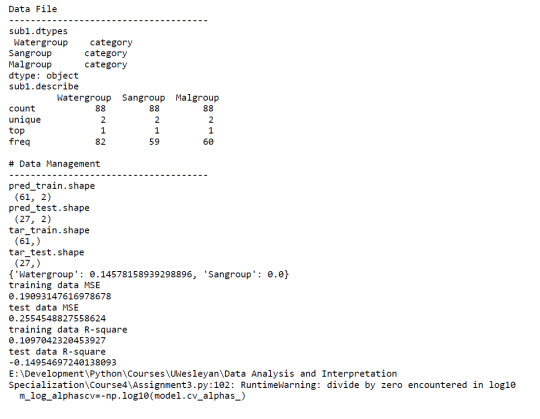
A lasso regression analysis was conducted to identify a subset of variables from 2 categorical predictor variables that best predicted a categorical response variable measuring high or low Malaria cases. Categorical predictors included Water and Sanitation Access. All predictor variables were standardized to have a mean of zero and a standard deviation of one.

Data were randomly split into a training set that included 70% of the observations (N=61) and a test set that included 30% of the observations (N=27). The least angle regression algorithm with k=10 fold cross validation was used to estimate the lasso regression model in the training set, and the model was validated using the test set. The change in the cross validation average (mean) squared error at each step was used to identify the best subset of predictor variables.

Of the 2 predictor variables, 1 was retained in the selected model. During the estimation process,water access was most strongly associated with Malaria cases.

[captaindentex]

Machine Learning for Data Analysis: Assignement 2

#Loading Libraries import numpy as np import pandas as pd import matplotlib import matplotlib.pyplot as plt import scipy.stats as sp import datetime as dt import time as tm import os import csv import seaborn import pydotplus import sklearn.metrics import statsmodels.api as sm import statsmodels.formula.api as smf import statsmodels.stats.multicomp as multi from pandas import Series, DataFrame from io import StringIO from IPython.display import Image from scipy.spatial.distance import cdist from sklearn import tree from sklearn import datasets from sklearn import preprocessing from sklearn.model_selection import train_test_split from sklearn.tree import DecisionTreeClassifier from sklearn.metrics import classification_report from sklearn.metrics import mean_squared_error from sklearn.ensemble import ExtraTreesClassifier from sklearn.ensemble import RandomForestClassifier from sklearn.linear_model import LassoLarsCV from sklearn.cluster import KMeans from sklearn.decomposition import PCA

print('') print('Data File') print('-------------------------------------') file='datamal.csv' data=pd.read_csv(file,low_memory=False) #data.columns=map(str.upper,data.columns) pd.set_option('display.float_format',lambda x: '%f' %x) data['Water']=data['Water'].apply(pd.to_numeric, errors='coerce') #Explanatory variable data['Sanitation']=data['Sanitation'].apply(pd.to_numeric, errors='coerce') #Explanatory variable data['Malaria']=data['Malaria'].apply(pd.to_numeric, errors='coerce') #Response variable

#Remove missing values subdata=data[['Country', 'Water', 'Sanitation', 'Malaria']].dropna()

#Grouping explanatory variables subdata['Watergroup']=pd.cut(subdata.Water, [0.00, 0.50, 1.00],labels=[0,1]) subdata['Sangroup']=pd.cut(subdata.Sanitation, [0.00, 0.50, 1.00],labels=[0,1]) subdata['Malgroup']=pd.cut(subdata.Malaria, [0.00, 10000.00, 12000000.00],labels=[0,1])

#Remove missing values sub1=subdata[['Watergroup','Sangroup','Malgroup']].dropna() print('sub1.dtypes\n',sub1.dtypes) print('sub1.describe\n',sub1.describe())

print('') print('Modeling and Prediction') print('-------------------------------------') #Split into training and testing sets predictors=sub1[['Watergroup','Sangroup']]

targets=sub1.Malgroup

pred_train, pred_test, tar_train, tar_test=train_test_split(predictors, targets, test_size=0.4)

print('pred_train.shape\n',pred_train.shape) print('pred_test.shape\n',pred_test.shape) print('tar_train.shape\n',tar_train.shape) print('tar_test.shape\n',tar_test.shape)

#Build model on training data classifier=RandomForestClassifier(n_estimators=3) classifier=classifier.fit(pred_train,tar_train) predictions=classifier.predict(pred_test) print('metrics.confusion_matrix\n',sklearn.metrics.confusion_matrix(tar_test,predictions)) print('metrics.accuracy_score\n',sklearn.metrics.accuracy_score(tar_test, predictions))

# fit an Extra Trees model to the data model=ExtraTreesClassifier() model.fit(pred_train,tar_train)

# display the relative importance of each attribute print(model.feature_importances_)

print('Running a different number of trees and see the effect of that on the accuracy of the prediction') trees=range(3) accuracy=np.zeros(3)

for idx in range(len(trees)):   classifier=RandomForestClassifier(n_estimators=idx + 1)   classifier=classifier.fit(pred_train,tar_train)   predictions=classifier.predict(pred_test)   accuracy[idx]=sklearn.metrics.accuracy_score(tar_test, predictions)

plt.cla() plt.plot(trees, accuracy)

Random forest analysis was performed to evaluate the importance of a series of explanatory variables in predicting a  binary, categorical response variable taken from the Gapminder Dataset. The total number of observations is 88 so this means a total of 52 (60%) train values and 36 (40%) test values

The explanatory variable with the highest relative importance scores was  Water Access. The accuracy of the random forest was 75%, with the subsequent growing of multiple trees rather than a single tree,lightly reducing the overall accuracy of the model, and suggesting that interpretation of a single decision tree may be appropriate.

[captaindentex]

Machine Learning for Data Analysis: Assignement 1

#Loading Libraries import numpy as np import pandas as pd import matplotlib import matplotlib.pyplot as plt import scipy.stats as sp import datetime as dt import time as tm import os import csv import seaborn import pydotplus import sklearn.metrics import statsmodels.api as sm import statsmodels.formula.api as smf import statsmodels.stats.multicomp as multi from pandas import Series, DataFrame from io import StringIO from IPython.display import Image from scipy.spatial.distance import cdist from sklearn import tree from sklearn import datasets from sklearn import preprocessing from sklearn.model_selection import train_test_split from sklearn.tree import DecisionTreeClassifier from sklearn.metrics import classification_report from sklearn.metrics import mean_squared_error from sklearn.ensemble import ExtraTreesClassifier from sklearn.ensemble import RandomForestClassifier from sklearn.linear_model import LassoLarsCV from sklearn.cluster import KMeans from sklearn.decomposition import PCA

print('') print('Data File') print('-------------------------------------') file='datamal.csv' data=pd.read_csv(file,low_memory=False) #data.columns=map(str.upper,data.columns) pd.set_option('display.float_format',lambda x: '%f' %x) data['Water']=data['Water'].apply(pd.to_numeric, errors='coerce') #Explanatory variable data['Sanitation']=data['Sanitation'].apply(pd.to_numeric, errors='coerce') #Explanatory variable data['Malaria']=data['Malaria'].apply(pd.to_numeric, errors='coerce') #Response variable

#Remove missing values subdata=data[['Country', 'Water', 'Sanitation', 'Malaria']].dropna()

#Grouping explanatory variables subdata['Watergroup']=pd.cut(subdata.Water, [0.00, 0.50, 1.00],labels=[0,1]) subdata['Sangroup']=pd.cut(subdata.Sanitation, [0.00, 0.50, 1.00],labels=[0,1]) subdata['Malgroup']=pd.cut(subdata.Malaria, [0.00, 10000.00, 12000000.00],labels=[0,1])

#Remove missing values sub1=subdata[['Watergroup','Sangroup','Malgroup']].dropna() print('sub1.dtypes\n',sub1.dtypes) print('sub1.describe\n',sub1.describe())

print('') print('Modeling and Prediction') print('-------------------------------------') #Split into training and testing sets predictors=sub1[['Watergroup','Sangroup']]

targets=sub1.Malgroup

pred_train, pred_test, tar_train, tar_test=train_test_split(predictors, targets, test_size=0.4)

print('pred_train.shape\n',pred_train.shape) print('pred_test.shape\n',pred_test.shape) print('tar_train.shape\n',tar_train.shape) print('tar_test.shape\n',tar_test.shape)

#Build model on training data classifier=DecisionTreeClassifier() classifier=classifier.fit(pred_train,tar_train)

predictions=classifier.predict(pred_test)

print('metrics.confusion_matrix\n',sklearn.metrics.confusion_matrix(tar_test,predictions)) print('metrics.accuracy_score\n',sklearn.metrics.accuracy_score(tar_test, predictions))

#Displaying the decision tree out=StringIO() tree.export_graphviz(classifier, out_file=out) graph=pydotplus.graph_from_dot_data(out.getvalue()) Image(graph.create_png()) graph.write_pdf("tree1.pdf")

Decision tree analysis was performed to test nonlinear relationships among a series of explanatory variables and a binary, categorical response variable taken from the Gapminder Dataset. The total number of observations is 88 so this means a total of 52 (60%) train values and 36 (40%) test values

The following explanatory variables were included as possible predictors to a classification tree model evaluating Malaria cases (my response - target variable), Water Access and Sanitation Access

The resulting tree starts with my first explanatory variable which is Water Access. If the value of Water Access is less than 0.5 (Low Water Access or less than 50%) then we got 2 observations where there are two cases of Low Malaria and no case of High Malaria

The rest 50 on the side right show observations with high Water Access. Then there is another split for the Sanitation Access variable where 20 observations are on low Sanitation Access and 30 on high Sanitation Access. There we can see that there are 5 cases of Low Malaria and 9 of High Malaria in regions with High Water and Low Sanitation whereas there  are 15 cases of Low Malaria and 21 of High Malaria in regions with High Water and High Sanitation Access

[captaindentex]

Regression Modelling in Practice: Assignement 4

#Loading Libraries import numpy as np import pandas as pd import matplotlib import matplotlib.pyplot as plt import scipy.stats as sp import datetime as dt import time as tm import csv import seaborn import statsmodels.api as sm import statsmodels.formula.api as smf import statsmodels.stats.multicomp as multi

print('') print('Data file') print('-------------------------------------') file='datamal.csv' data=pd.read_csv(file,low_memory=False) #data.columns=map(str.upper,data.columns) pd.set_option('display.float_format',lambda x: '%f' %x) data['Water']=data['Water'].apply(pd.to_numeric, errors='coerce') #Explanatory variable data['Sanitation']=data['Sanitation'].apply(pd.to_numeric, errors='coerce') #Explanatory variable data['Malaria']=data['Malaria'].apply(pd.to_numeric, errors='coerce') #Response variable

#Remove missing values subdata=data[['Country', 'Water', 'Sanitation', 'Malaria']].dropna()

print('') print('Step 1') print('-------------------------------------') #Grouping explanatory variables subdata['Watergroup']=pd.cut(subdata.Water, [0.00, 0.50, 1.00],labels=["Low","High"]) subdata['Sangroup']=pd.cut(subdata.Sanitation, [0.00, 0.50, 1.00],labels=["Low","High"])

def Mal (row):   if row['Malaria'] <= 10000.00:      return 0   else:      return 1

subdata['Mal'] = subdata.apply (lambda row: Mal (row),axis=1)

#Remove missing values sub1=subdata[['Watergroup','Sangroup','Mal']].dropna()

print('') print('Logistic Regression') lreg=smf.logit(formula = 'Mal ~ Watergroup + Sangroup', data = sub1).fit() print(lreg.summary())

print("Odds Ratios") params=lreg.params conf=lreg.conf_int() conf['OR']=params conf.columns=['Lower CI', 'Upper CI', 'OR'] print(np.exp(conf))

Step 1) In this assignment i have chosen to examine the relationship between three quantitative variables from the Gapminder Dataset. My explanatory variable is the overall Water Access of a population and my response variable is the recorded Malaria Cases of that population grouped in the categories 0(zero) for countries with less than 10.000 cases and 1(one) for more . I also examine the overall Sanitation Access as o confounding variable  My goal is to see if there is a connection between those so I tested a logistic regression model

The p-values for Water  Access is less than 0.05  which shows that we can reject the null hypothesis so there is  connection between these variables :

The odds on having significant Malaria cases (more than 10.000) were 7.2 times greater for populations with high  Water Access. On the odds at Sanitation Access is less than 1 that means for high Sanitation Access less Malaria Cases are less likely

Step 2) The above results do not give support to my hypothesis that Malaria cases are associated with Water  Access 

Step 3)  Since p-values remain non significant we can say that there is no evidence of confounding

[captaindentex]

Regression Modelling in Practice: Assignement 3

#Loading Libraries import numpy as np import pandas as pd import matplotlib import matplotlib.pyplot as plt import scipy.stats as sp import datetime as dt import time as tm import csv import seaborn import statsmodels.api as sm import statsmodels.formula.api as smf import statsmodels.stats.multicomp as multi

print('') print('Data file') print('-------------------------------------') file='datamal.csv' data=pd.read_csv(file,low_memory=False) #data.columns=map(str.upper,data.columns) pd.set_option('display.float_format',lambda x: '%f' %x) #Explanatory variable data['Water']=data['Water'].apply(pd.to_numeric, errors='coerce') #Explanatory variable data['Sanitation']=data['Sanitation'].apply(pd.to_numeric, errors='coerce') #Response variable data['Malaria']=data['Malaria'].apply(pd.to_numeric, errors='coerce')

#Remove missing values subdata=data[['Country', 'Water', 'Sanitation', 'Malaria']].dropna()

#Center quantitative IVs for regression analysis subdata['Water_c'] = (subdata['Water'] - subdata['Water'].mean()) subdata['Sanitation_c'] = (subdata['Sanitation'] - subdata['Sanitation'].mean())

print('') print('Step 1') print('Multiple regression analysis') print('-------------------------------------') reg1l=smf.ols('Malaria ~ Water_c + Sanitation_c', data=subdata).fit() print(reg1l.summary())

print('') print('Model evaluation - Water') print('-------------------------------------') # q-q plot fig1=sm.qqplot(reg1l.resid, line='r')

# simple plot of residuals plt.figure() stdres=pd.DataFrame(reg1l.resid_pearson) plt.plot(stdres, 'o', ls='None') l=plt.axhline(y=0, color='r') plt.ylabel('Standardized Residual') plt.xlabel('Observation Number') plt.plot()

# additional regression diagnostic plots fig=plt.figure() fig2=sm.graphics.plot_regress_exog(reg1l,  "Sanitation_c", fig=fig)

# leverage plot fig3=sm.graphics.influence_plot(reg1l, size=8) print(fig3)

Step 1) In this assignment i have chosen to examine the relationship between three quantitative variables from the Gapminder Dataset. My explanatory variable is the overall Water Access of a population and my response variable is the recorded Malaria Cases of that population. I also examine the overall Sanitation Access as o confounding variable  My goal is to see if there is a connection between those. I have tested a multiple regression model and the main characteristics are the following:

No of Observations = 88

F-Statistic = 0.3744

p-value = 0.689

R-squared = 0.009

The p-values for Water and Sanitation Access (centerd variables) are both greater than 0.05 while both of the parameter estimates are positive which shows that we cannot reject the null hypothesis so there is no connection between these variables :

Step 2) The above results do not give support to my hypothesis that Malaria cases are associated with Water and Sanitation Access

Step 3)  Since p-values remain non significant we can say that there is no evidence of confounding

Step 4) First i have created a qq plot to evaluate the assumption that the residuals are normally distributed. From the graph we can see that the points do not follow a straight lines which means that the residuals are not normally distributed

Second i have created a simple plot of residuals where it is clear that most residuals do not fall within a standard deviation but are mostlhy in the -1 region. Moreover there are many residuals that are more thatn two s.d. from the mean which measn that there may be outliers and the fact that there are two residuals thar are in the 5 s.d.region means that there are extreme outliers.

I created additional diagnostic plots to determine how Sanitation Access contributes to the fit of the model From the partial regression plot we can see that there is a linear relationship between Sanitation access and Malaria cases

Last i have created a leverage plot to identify observations that have an unusually large influence on the estimation of the predicted value of the response variable. From the graph we can see that there are outliers and also high leveraged values

[captaindentex]

Regression Modelling in Practice: Assignement 2

#Loading Libraries import numpy as np import pandas as pd import matplotlib import matplotlib.pyplot as plt import scipy.stats as sp import datetime as dt import time as tm import csv import seaborn import statsmodels.api as sm import statsmodels.formula.api as smf import statsmodels.stats.multicomp as multi

print('') print('Data file') print('-------------------------------------') file='datamal.csv' data=pd.read_csv(file,low_memory=False) #data.columns=map(str.upper,data.columns) pd.set_option('display.float_format',lambda x: '%f' %x) #Explanatory variable data['Water']=data['Water'].apply(pd.to_numeric, errors='coerce') #Response variable data['Malaria']=data['Malaria'].apply(pd.to_numeric, errors='coerce')

#Remove missing values subdata=data[['Country', 'Water', 'Malaria']].dropna()

print('') print('Step 1') print('Center quantitative IVs for regression analysis') print('-------------------------------------') subdata['Water_c'] = (subdata['Water'] - subdata['Water'].mean()) print(subdata['Water_c'].mean())

print('') print('Step 2') print("OLS regression model for the association between Water Access and Malaria Cases") print('-------------------------------------') reg=smf.ols('Malaria ~ Water_c', data=subdata).fit() print(reg.summary())

In this assignment i have chosen to examine the relationship between two quantitative variables from the Gapminder Dataset. My explanatory variable is the overall Water Access of a population and my response variable is the recorded Malaria Cases of that population. My goal is to see if there is a connection between those.

Step 1) Since I have a quantitative explanatory variable, I center it so that the mean = 0  by subtracting the mean, From the calculation of the mean i get 1.54e-16 which means that it is real close to zero

Step 2) I have tested a basic linear regression model and the main characteristics are the following:

No of Observations = 89

F-Statistic = 0.8038

p-value = 0.372

R-squared = 0.009

The parameter estimates are the following:

Water coeff (b1) = 9.52e+05

Intercept (b0) = 8.55e+05

so my equation is Malaria_Cases=9.52e+05Water_Access + 8.55e+05

The p-value being significantly more than 0.005 indicated that water access is not significantly and positively associated with malaria cases  

[captaindentex]

Regression Modelling in Practice: Assignement 1

Step 1)

a)The study population comes from the samples of the national population of each country who participated in the general census

b)The level of analysis is in population groups that correspond to each country of the world

c)The number of observations is 99

d)My sample comes from all people who participate in national census 

Step 2)

a) Data were generated by surveys

b)Original purpose of the data collection was for census reasons

c)Data were collected during the national census procedure

d)Data were collected during the 2003 period

e)Data are worldwide

Step 3)

a)My explanatory variables measure the overall access of a population to water and sanitation facilities while my response variable is the reported malaria cases of the population

b)For my explanatory variables my response scales is 0-100% while for my response variable it is the absolute number of cases

c)My variables were managed in a csv format

[captaindentex]

Data Analysis Tools: Assignement 4

#Loading Libraries import numpy as np import pandas as pd import matplotlib import matplotlib.pyplot as plt import scipy.stats as sp import datetime as dt import time as tm import csv import seaborn import statsmodels.formula.api as smf import statsmodels.stats.multicomp as multi

print('') print('Data File') print('-------------------------------------') # Open csv file file='datamal.csv' data=pd.read_csv(file,low_memory=False) pd.set_option('display.float_format',lambda x: '%f' %x)

#Explanatory variable - Covert to numeric value data['Water']=data['Water'].apply(pd.to_numeric, errors='coerce') #Explanatory variable - Covert to numeric value data['Sanitation']=data['Sanitation'].apply(pd.to_numeric, errors='coerce') #Response variable - Covert to numeric value data['Malaria']=data['Malaria'].apply(pd.to_numeric, errors='coerce')

#Removing missing data subdata=data[['Country', 'Water', 'Sanitation', 'Malaria']].dropna()

print(sp.pearsonr(subdata['Water'], subdata['Malaria']))

def San (row):   if row['Sanitation'] <= 0.25:      return 1   elif row['Sanitation'] <= 0.50 :      return 2   elif row['Sanitation'] > 0.50:      return 3

subdata['San'] = subdata.apply (lambda row: San (row),axis=1)

chk=subdata['San'].value_counts(sort=False, dropna=False) print(chk)

sub1=subdata[(subdata['San']== 1)] sub2=subdata[(subdata['San']== 2)] sub3=subdata[(subdata['San']== 3)]

print ('association between Water Access and Malaria Cases for LOW Sanitation Access') print (sp.pearsonr(sub1['Water'], sub1['Malaria'])) print ('       ') print ('association between Water Access and Malaria Cases for MIDDLE Sanitation Access') print (sp.pearsonr(sub2['Water'], sub2['Malaria'])) print ('       ') print ('association between Water Access and Malaria Cases for HIGH Sanitation Access') print (sp.pearsonr(sub3['Water'], sub3['Malaria'])) #%% plt.figure() scat1=seaborn.regplot(x="Water", y="Malaria", data=sub1) plt.xlabel('Water Access') plt.ylabel('Malaria Cases') plt.title('Scatterplot for the Association Between Water Access and Malaria Cases for LOW Sanitation Access') plt.plot() #%% plt.figure() scat2=seaborn.regplot(x="Water", y="Malaria", data=sub2) plt.xlabel('Water Access') plt.ylabel('Malaria Cases') plt.title('Scatterplot for the Association Between Water Access and Malaria Cases for MIDDLE Sanitation Access') plt.plot() #%% plt.figure() scat3=seaborn.regplot(x="Water", y="Malaria", data=sub3) plt.xlabel('Water Access') plt.ylabel('Malaria Cases') plt.title('Scatterplot for the Association Between Water Access and Malaria Cases for HIGH Sanitation Access') plt.plot()

When examining the association between malaria cases (quantitative response) and water access (quantitative explanatory),i inserted sanitation access as a categorical (three levels low, middle, high) moderator . Moderation testing in the context of correlation reveals that high p-vales (0.46, 0.065 and 0.369 respectively show that there is no connection between those three variables)

[captaindentex]

Data Analysis Tools: Assignement 3

#Loading Libraries import numpy as np import pandas as pd import matplotlib import matplotlib.pyplot as plt import scipy.stats as sp import datetime as dt import time as tm import csv import seaborn import statsmodels.formula.api as smf import statsmodels.stats.multicomp as multi

print('') print('Data File') print('-------------------------------------') # Open csv file file='datamal.csv' data=pd.read_csv(file,low_memory=False) pd.set_option('display.float_format',lambda x: '%f' %x)

#Explanatory variable - Covert to numeric value data['Water']=data['Water'].apply(pd.to_numeric, errors='coerce') #Explanatory variable - Covert to numeric value data['Sanitation']=data['Sanitation'].apply(pd.to_numeric, errors='coerce') #Response variable - Covert to numeric value data['Malaria']=data['Malaria'].apply(pd.to_numeric, errors='coerce')

#Removing missing data subdata=data[['Country', 'Water', 'Sanitation', 'Malaria']].dropna()

print('') print('Water Access - Sanitation Access Correlation') print('-------------------------------------') print(sp.pearsonr(subdata['Water'], subdata['Sanitation']))

plt.figure() seaborn.regplot(x='Water', y='Sanitation', fit_reg=True, data=subdata) plt.title('Water Access - Sanitation Access Correlation') plt.xlabel('Water Access') plt.ylabel('Sanitation Access') plt.plot()

When examining the association between sanitation access (quantitative response) and water access (quantitative explanatory), a pearson correlation test revealed that a positive and close to 1 r  (0.873) and a significant p-value (1,34e-28) shows that there is a strong relationship between these two variables meaning that countries with high water access have also high sanitation access

[captaindentex]

Data Analysis Tools: Assignement 2

#Loading Libraries import numpy as np import pandas as pd import matplotlib import matplotlib.pyplot as plt import scipy.stats as sp import datetime as dt import time as tm import csv import seaborn import statsmodels.formula.api as smf import statsmodels.stats.multicomp as multi

print('') print('Data File') print('-------------------------------------') # Open csv file file='datamal.csv' data=pd.read_csv(file,low_memory=False) pd.set_option('display.float_format',lambda x: '%f' %x)

#Explanatory variable - Covert to numeric value data['Water']=data['Water'].apply(pd.to_numeric, errors='coerce') #Explanatory variable - Covert to numeric value data['Sanitation']=data['Sanitation'].apply(pd.to_numeric, errors='coerce') #Response variable - Covert to numeric value data['Malaria']=data['Malaria'].apply(pd.to_numeric, errors='coerce')

#Removing missing data subdata=data[['Country', 'Water', 'Sanitation', 'Malaria']].dropna()

#Grouping explanatory variables subdata['Watergroup']=pd.cut(subdata.Water, [0.00, 0.25, 0.50, 0.75, 1.00],labels=["0-25%","25-50%","50-75%","75-100%"]) subdata['Sangroup']=pd.cut(subdata.Sanitation, [0.00, 0.25, 0.50, 0.75, 1.00],labels=["0-25%","25-50%","50-75%","75-100%"])

print('') print('contingency table of observed counts') print('-------') ct=pd.crosstab(subdata['Watergroup'], subdata['Sangroup']) print(ct)

print('') print('column percentages') print('-------') colsum=ct.sum(axis=0) colpct=ct/colsum print(colpct)

print('') print('chi-square value, p value, expected counts') print('-------') cs=sp.chi2_contingency(ct) print(cs)

When examining the association between sanitation access (categorical response) andwater access (categorical explanatory), a chi-square test of independence revealed that a significant chi-square value (62.63) and a very low p-value (4.17e-10) shows that there is a significant relationship between these two variables meaning that countries with high water access have also high sanitation access

[captaindentex]

Data Analysis Tools: Assignement 1

#Loading Libraries import numpy as np import pandas as pd import matplotlib import matplotlib.pyplot as plt import scipy.stats as sp import datetime as dt import time as tm import csv import seaborn import statsmodels.formula.api as smf import statsmodels.stats.multicomp as multi

print('') print('Data File') print('-------------------------------------') # Open csv file file='datamal.csv' data=pd.read_csv(file,low_memory=False) pd.set_option('display.float_format',lambda x: '%f' %x)

#Explanatory variable - Covert to numeric value data['Water']=data['Water'].apply(pd.to_numeric, errors='coerce') #Explanatory variable - Covert to numeric value data['Sanitation']=data['Sanitation'].apply(pd.to_numeric, errors='coerce') #Response variable - Covert to numeric value data['Malaria']=data['Malaria'].apply(pd.to_numeric, errors='coerce')

#Removing missing data subdata=data[['Country', 'Water', 'Sanitation', 'Malaria']].dropna()

#Grouping explanatory variables subdata['Watergroup']=pd.cut(subdata.Water, [0.20, 0.50, 0.80, 1.00],labels=["Low","Medium","High"])

print('') print('Water Access - Malaria Cases') print('-------------------------------------') sub1=subdata[['Malaria', 'Watergroup']].dropna() print('') print('ANOVA: Test') print('-------') model1=smf.ols(formula='Malaria ~ C(Watergroup)', data=sub1).fit() print(model1.summary())

print ('means for Malaria Cases by Water Access status') m1=sub1.groupby('Watergroup').mean() print(m1)

print ('standard deviations Malaria Cases by Water Access status') sd1=sub1.groupby('Watergroup').std() print(sd1)

print('') print('Post hoc Tests for ANOVA') print('-------') mc1=multi.MultiComparison(sub1['Malaria'], sub1['Watergroup']) res1=mc1.tukeyhsd() print(res1.summary())

When examining the association between malaria cases (quantitative response) and water access (in three groups - low, medium, high- categorical explanatory) from the gapminder dataset, an Analysis of Variance (ANOVA) revealed that there is a significant p value (p=0.408) which is enough to accept the null hypothesis that there is no connection between water access and malaria cases. However the means were expected to be equal but as anyoyne can see there is a significant difference between each group. So i ran a post hoc test   that shows it is false to reject the null hypothesis and there is indeed no connection betwwwn these two variables

[captaindentex]

Data Management & Visualization: Assignement 4

Loading Libraries import numpy as np import pandas as pd import matplotlib import matplotlib.pyplot as plt import scipy.stats as sp import datetime as dt import time as tm import csv import seaborn

print('') print('Data File') print('-------------------------------------') # Open csv file file='datamal.csv' data=pd.read_csv(file,low_memory=False) pd.set_option('display.float_format',lambda x: '%f' %x)

#Explanatory variable - Covert to numeric value data['Water']=data['Water'].apply(pd.to_numeric, errors='coerce') #Explanatory variable - Covert to numeric value data['Sanitation']=data['Sanitation'].apply(pd.to_numeric, errors='coerce') #Response variable - Covert to numeric value data['Malaria']=data['Malaria'].apply(pd.to_numeric, errors='coerce')

#Removing missing data subdata=data[['Country', 'Water', 'Sanitation', 'Malaria']].dropna()

#Grouping Water values subdata['Watergroup']=pd.cut(subdata.Water, [0.20, 0.40, 0.60, 0.80, 1.00]) #Grouping Sanitation values subdata['Sangroup']=pd.cut(subdata.Sanitation, [0.00, 0.20, 0.40, 0.60, 0.80, 1.00]) #Grouping Malaria values subdata['Malgroup']=pd.cut(subdata.Malaria, [0, 1e3, 1e4, 1e5, 1e6, 1e7, 1e8])

print('') print('Bivariate Graphs') print('-------------------------------------') plt.figure() seaborn.factorplot(x='Watergroup', y='Malaria', data=subdata, kind="bar", ci=None) plt.xlabel('Water') plt.ylabel('Malaria') plt.plot()

plt.figure() seaborn.factorplot(x='Sangroup', y='Malaria', data=subdata, kind="bar", ci=None) plt.xlabel('Water') plt.ylabel('Malaria') plt.plot()

print('') print('Scatterplots') print('-------------------------------------') plt.figure() scat1 = seaborn.regplot(x="Water",y="Malaria", data=subdata) plt.ylabel('Malaria Cases') plt.xlabel('Water Access') plt.title('Scatterplot for the Association Between Water Access and Malaria Cases') plt.plot()

plt.figure() scat1 = seaborn.regplot(x="Sanitation",y="Malaria", data=subdata) plt.ylabel('Malaria Cases') plt.xlabel('Sanitation Access') plt.title('Scatterplot for the Association Between Sanitation Access and Malaria Cases') plt.plot()

The bivariate graph of Water access vs Malaria cases. It shows that higher water access means higher malaria cases which comes against our hypothesis

The bivariate graph of Sanitation access vs Malaria cases. It shows that higher  higher malaria cases occur when sanitation access is 60%-80% which comes against our hypothesis

The graph above plots the water (a1) and sanitation (a2) access of a country to the country’s reported malaria cases. We can see that the scatter graph does not show a clear relationship/trend between the two variables.

[captaindentex]

Data Management & Visualization: Assignement 3

#Loading Libraries import numpy as np import pandas as pd import matplotlib import matplotlib.pyplot as plt import scipy.stats as sp import datetime as dt import time as tm import csv import seaborn

print('') print('Data File') print('-------------------------------------') # Open csv file file='datamal.csv' data=pd.read_csv(file,low_memory=False) pd.set_option('display.float_format',lambda x: '%f' %x)

#Explanatory variable - Covert to numeric value data['Water']=data['Water'].apply(pd.to_numeric, errors='coerce') #Explanatory variable - Covert to numeric value data['Sanitation']=data['Sanitation'].apply(pd.to_numeric, errors='coerce') #Response variable - Covert to numeric value data['Malaria']=data['Malaria'].apply(pd.to_numeric, errors='coerce')

#Removing missing data subdata=data[['Country', 'Water', 'Sanitation', 'Malaria']].dropna()

#Grouping Water values print('Water quartile split') subdata['Watergroup1']=pd.qcut(subdata.Water, 4, labels=["0%","25%","50%","75%"]) wg1=subdata['Watergroup1'].value_counts(sort=False, dropna=True) print(wg1) print('Water customized split') subdata['Watergroup2']=pd.cut(subdata.Water, [0.20, 0.40, 0.60, 0.80, 1.00]) wg2=subdata['Watergroup2'].value_counts(sort=False, dropna=True) print(wg2)

print('Crosstabs evaluating Watergroup1') print(pd.crosstab(subdata['Watergroup1'], subdata['Water'])) print('Crosstabs evaluating Watergroup2') print(pd.crosstab(subdata['Watergroup2'], subdata['Water']))

#Grouping Sanitation values print('Sanitation quartile split') subdata['Sangroup1']=pd.qcut(subdata.Sanitation, 4, labels=["0%","25%","50%","75%"]) sg1=subdata['Sangroup1'].value_counts(sort=False, dropna=True) print(sg1) print('Sanitation customized split') subdata['Sangroup2']=pd.cut(subdata.Sanitation, [0.00, 0.20, 0.40, 0.60, 0.80, 1.00]) sg2=subdata['Sangroup2'].value_counts(sort=False, dropna=True) print(sg2)

print('Crosstabs evaluating Sangroup1') print(pd.crosstab(subdata['Sangroup1'], subdata['Sanitation'])) print('Crosstabs evaluating Sangroup2') print(pd.crosstab(subdata['Sangroup2'], subdata['Sanitation']))

#Grouping Malaria values print('Malaria quartile split') subdata['Malgroup1']=pd.qcut(subdata.Malaria, 4, labels=["0%","25%","50%","75%"]) mg1=subdata['Malgroup1'].value_counts(sort=False, dropna=True) print(mg1) print('Malaria customized split') subdata['Malgroup2']=pd.cut(subdata.Malaria, [0, 1e3, 1e4, 1e5, 1e6, 1e7, 1e8]) mg2=subdata['Malgroup2'].value_counts(sort=False, dropna=True) print(mg2)

print('Crosstabs evaluating Malgroup1') print(pd.crosstab(subdata['Malgroup1'], subdata['Malaria'])) print('Crosstabs evaluating Malgroup2') print(pd.crosstab(subdata['Malgroup2'], subdata['Malaria']))

Data File ------------------------------------- Water quartile split 0%     22 25%    22 50%    22 75%    22 Name: Watergroup1, dtype: int64 Water customized split (0.2, 0.4]     3 (0.4, 0.6]    15 (0.6, 0.8]    11 (0.8, 1.0]    59 Name: Watergroup2, dtype: int64 Crosstabs evaluating Watergroup1 Water        0.233000  0.356000  0.385000  ...  0.998000  0.999000  1.000000 Watergroup1                                ...                               0%                  1         1         1  ...         0         0         0 25%                 0         0         0  ...         0         0         0 50%                 0         0         0  ...         0         0         0 75%                 0         0         0  ...         1         1        12

[4 rows x 70 columns] Crosstabs evaluating Watergroup2 Water        0.233000  0.356000  0.385000  ...  0.998000  0.999000  1.000000 Watergroup2                                ...                               (0.2, 0.4]          1         1         1  ...         0         0         0 (0.4, 0.6]          0         0         0  ...         0         0         0 (0.6, 0.8]          0         0         0  ...         0         0         0 (0.8, 1.0]          0         0         0  ...         1         1        12

[4 rows x 70 columns] Sanitation quartile split 0%     22 25%    22 50%    22 75%    22 Name: Sangroup1, dtype: int64 Sanitation customized split (0.0, 0.2]    13 (0.2, 0.4]    12 (0.4, 0.6]     8 (0.6, 0.8]     8 (0.8, 1.0]    47 Name: Sangroup2, dtype: int64 Crosstabs evaluating Sangroup1 Sanitation  0.041100  0.054900  0.097900  ...  0.998000  0.999000  1.000000 Sangroup1                                 ...                               0%                 1         1         1  ...         0         0         0 25%                0         0         0  ...         0         0         0 50%                0         0         0  ...         0         0         0 75%                0         0         0  ...         2         1         7

[4 rows x 79 columns] Crosstabs evaluating Sangroup2 Sanitation  0.041100  0.054900  0.097900  ...  0.998000  0.999000  1.000000 Sangroup2                                 ...                               (0.0, 0.2]         1         1         1  ...         0         0         0 (0.2, 0.4]         0         0         0  ...         0         0         0 (0.4, 0.6]         0         0         0  ...         0         0         0 (0.6, 0.8]         0         0         0  ...         0         0         0 (0.8, 1.0]         0         0         0  ...         2         1         7

[5 rows x 79 columns] Malaria quartile split 0%     22 25%    22 50%    22 75%    22 Name: Malgroup1, dtype: int64 Malaria customized split (0.0, 1000.0]                15 (1000.0, 10000.0]            13 (10000.0, 100000.0]          21 (100000.0, 1000000.0]        21 (1000000.0, 10000000.0]      16 (10000000.0, 100000000.0]     2 Name: Malgroup2, dtype: int64 Crosstabs evaluating Malgroup1 Malaria    6.000000         7.000000         ...  11000000.000000  11400000.000000 Malgroup1                                    ...                                   0%                       1                1  ...                0                0 25%                      0                0  ...                0                0 50%                      0                0  ...                0                0 75%                      0                0  ...                1                1

[4 rows x 88 columns] Crosstabs evaluating Malgroup2 Malaria                    6.000000         ...  11400000.000000 Malgroup2                                   ...                 (0.0, 1000.0]                            1  ...                0 (1000.0, 10000.0]                        0  ...                0 (10000.0, 100000.0]                      0  ...                0 (100000.0, 1000000.0]                    0  ...                0 (1000000.0, 10000000.0]                  0  ...                0 (10000000.0, 100000000.0]                0  ...                1

[6 rows x 88 columns]

I split the responses for Water, Sanitation, and Malaria to  quartile and customized splits. Water is splitted to 20%-100%, Sanitation to 0%-100% and Malaria to 0 - 100.000.000 number of cases

[captaindentex]

Data Management & Visualization: Assignement 2

1)Python Code

#Loading Libraries import numpy as np import pandas as pd import matplotlib import matplotlib.pyplot as plt import scipy.stats as sp import datetime as dt import time as tm import csv import seaborn

# Open csv file file='datamal.csv' data=pd.read_csv(file,low_memory=False) pd.set_option('display.float_format',lambda x: '%f' %x)

#Explanatory variable - Covert to numeric value data['Water']=data['Water'].apply(pd.to_numeric, errors='coerce') #Explanatory variable - Covert to numeric value data['Sanitation']=data['Sanitation'].apply(pd.to_numeric, errors='coerce') #Response variable - Covert to numeric value data['Malaria']=data['Malaria'].apply(pd.to_numeric, errors='coerce')

#Removing missing data subdata=data[['Country', 'Water', 'Sanitation', 'Malaria']].dropna()

print('') print('Frequency Distributions') print('-------------------------------------') #Calculate Counts wat1=subdata.groupby('Water').size() #Calculate Percentages wat2=subdata.groupby('Water').size()/subdata.groupby('Water').size().sum() print('') print('Water - Counts') print('-------') print(wat1) print('') print('Water - Percentages') print('-------') print(wat2)

#Calculate Counts san1=subdata.groupby('Sanitation').size() #Calculate Percentages san2=subdata.groupby('Sanitation').size()/subdata.groupby('Sanitation').size().sum() print('') print('Sanitation - Counts') print('-------') print(san1) print('') print('Sanitation - Percentages') print('-------') print(san2)

#Calculate Counts mal1=subdata.groupby('Malaria').size() #Calculate Percentages mal2=subdata.groupby('Malaria').size()/subdata.groupby('Malaria').size().sum() print('') print('Malaria - Counts') print('-------') print(mal1) print('') print('Malaria - Percentages') print('-------') print(mal2)

2) Output

Frequency Distributions -------------------------------------

Water - Counts ------- Water 0.233000     1 0.356000     1 0.385000     1 0.410000     1 0.444000     1            .. 0.993000     2 0.997000     3 0.998000     1 0.999000     1 1.000000    12 Length: 70, dtype: int64

Water - Percentages ------- Water 0.233000   0.011364 0.356000   0.011364 0.385000   0.011364 0.410000   0.011364 0.444000   0.011364

0.993000   0.022727 0.997000   0.034091 0.998000   0.011364 0.999000   0.011364 1.000000   0.136364 Length: 70, dtype: float64

Sanitation - Counts ------- Sanitation 0.041100    1 0.054900    1 0.097900    1 0.098700    1 0.114000    1           .. 0.996000    1 0.997000    1 0.998000    2 0.999000    1 1.000000    7 Length: 79, dtype: int64

Sanitation - Percentages ------- Sanitation 0.041100   0.011364 0.054900   0.011364 0.097900   0.011364 0.098700   0.011364 0.114000   0.011364

0.996000   0.011364 0.997000   0.011364 0.998000   0.022727 0.999000   0.011364 1.000000   0.079545 Length: 79, dtype: float64

Malaria - Counts ------- Malaria 6.000000           1 7.000000           1 24.000000          1 29.000000          1 45.000000          1                  .. 3730000.000000     1 4860000.000000     1 5090000.000000     1 11000000.000000    1 11400000.000000    1 Length: 88, dtype: int64

Malaria - Percentages ------- Malaria 6.000000          0.011364 7.000000          0.011364 24.000000         0.011364 29.000000         0.011364 45.000000         0.011364

3730000.000000    0.011364 4860000.000000    0.011364 5090000.000000    0.011364 11000000.000000   0.011364 11400000.000000   0.011364 Length: 88, dtype: float64

3) Comments

Data from 88 countries  are taken from the Gapminder dataset and are combined in one csv file that displays the overall water and sanitation access of the population (%) and the total number of malaria cases as well.

Water access varies from 23% to 100%, sanitation from 41% to 100% while malaria cases from 6 to 11.400.000. We can see from the output that only 12 countries have 100% access to water and 7 have 100% access to sanitation. On the other hand malaria cases seems to be equaly distributed with no countries showing the same number of cases

[captaindentex]

Data Management & Visualization: Assignement 1

After looking through the GapMinder codebook, I have identified as a specific topic of interested the impact of Water Source Access on Malaria Cases. 

The datasets i have chosen to work with come from the Gapminder Foundation (www.gapminder.org) and are the following:

- 2003 at least basic water source overall access (%).

- 2003 reported malaria cases (number of cases)

My research question is to examine if there is an association between the basic water access through water infrastructure projects and the spread of malaria. More precisely my hypothesis is that in countries with high water infrastructure malaria cases reduce.

For this purpose i have made a codebook named that includes all my questions and variables.

As a second topic i would like to examine if sanitation access has any impact at  malaria spread. Therefore i have chosen one more dataset from the Gapminder codebook:

-2003  at least basic sanitation overall access (%)

and i make the hypothesis that  in countries with high sanitation infrastructure malaria cases reduce.

 The following journals describe research that has been done to examine the connection between water access and malaria cases