commercecurve

[commercecurve]

Protection Function in Microsoft Excel

What is the Protection Function or the Protect Range in Microsoft Excel?

The protect range function is a useful way to prevent other users of a workbook from altering data within a worksheet. By using this function, you can prevent the accidental or intentional modification or deletion of worksheets or cells within a worksheet. The protection function can further be enhanced by password protection. The use of a password allows you to strengthen the security of your workbook.

As the owner of the workbook, you can set the rules on what worksheets and cells are off limits for modification.

This can be a valuable function if you have created a workbook that you will be sharing with a third party and you want to ensure that they do not modify certain aspects of it. Without this feature used, you would have to manually check to see if they made modifications to the worksheet areas which you did not want modified. In this post I will demonstrate you how to use protect function in an Excel spreadsheet:

How to enable Protect Function in Microsoft Excel?

Practical Application of Protect function:

Steps to Enable Worksheet Protection: Step 1: In the Excel file, select the worksheet tab that you want to protect. Then go to the “Review” tab, and click “Protect Sheet”

Step 2: A prompt message will appear showing elements you want people to be able to change along with the requirement to enter a password.

There are several options available here with respect to what you would like to protect in the worksheet.

For instance, you may want to protect the worksheet but still allow the user to be able to

Select the cells of the worksheet to navigate it,

Format the cells,

Sort the data, and

Use PivotTable and PivotChart features while not modifying the data itself

In that case, you would multi-select those features in the below list and click OK.

Step 3: After pressing OK, the worksheet will now be protected. If you try to modify a protected worksheet, the below message notification will appear.

Step 4: You can also set range where you would like to allow someone to edit specific cells rather than the whole worksheet.

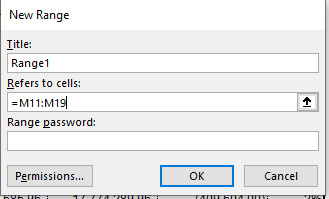
To do this, go to the “Review” tab, then click “Allow Edit Ranges” and click “New.” The below popup will appear. When this appears, you can give the editable range a title, and then in the “Refers to cells:” section, highlight the specific cells in the worksheet you would like to make editable.

If you do not enter a password, anyone will be able to edit that range. Then, you can protect the whole sheet again but this time the cells which you have setup as being allowed to edit will remain editable.

Note that on this screen you can also set a “range password.” This will allow someone to edit the range but only if they have the password. i.e. when they click on the cell and try to edit it, they will be prompted to enter a password.

This can be useful if you want to send a workbook to multiple individuals, protect the whole sheet, but only allow certain individuals to edit a certain part of the workbook. In that instance, you would need to provide those specific individuals with the range password you created.

Note that you can create multiple rules for “Allow edit ranges.” Below is the first one that was setup but you can go back to the “Allow Edit Ranges” at any time and create another editable range or modify or delete an existing editable range.

Step 5: You can also protect the entire workbook with a password instead of locking each individual tab.

I hope that helps. Please leave a comment below with any questions or suggestions. Thank you!

[commercecurve]

Screenshot insertion function in Microsoft Excel

What is the Screenshot function in Excel?

If you’re doing tutorials, walkthroughs or need to paste a screenshot In the Excel file to show a reference to something or support for something, the same can be done by using screenshot function of Excel. This function is occasionally more helpful than using the snipping tool because that tool occasionally closes an open window.

In this post I will explain you how to use screenshot insertion function with an example.

How to insert a Screenshot in Microsoft Excel sheet?

Below mentioned are the steps to insert a screenshot an Excel file:

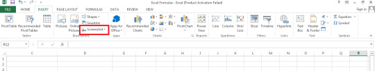
Navigate the home screen and go to the Insert tab

Click on screenshot

From the dropdown menu, select the screenshot of the window open on your desktop

Or click Screen Clipping from the drop down menu to select only a specific area of the screenshot to insert

Practical application of screenshot insertion function

Suppose the Accounting Staff of your organization would like to take a screenshot of the bank balance that shows up in online banking as at the end of the month. The bank statements have not been released yet by the bank so online access is available.

The Accounting staff opts to rather insert Screenshot of the balances, to do so following steps would be required to be followed:

Step 1: Navigate to home screen and go to the Insert tab, click on screenshot

Step 2: From the dropdown menu, select the screenshot of the window open on your desktop

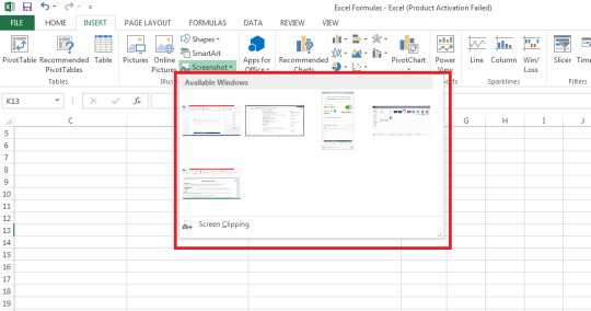
Step 3: Or click Screen Clipping from the drop-down menu to select only a specific area of the screenshot to insert

I hope that helps. Please leave a comment below with any questions or suggestions. Thank you!

[commercecurve]

Precedents and Dependents function in Microsoft Excel

What are “Trace Precedents” and “Trace Dependents” Function in Microsoft Excel?

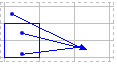
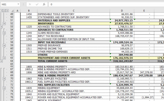
The precedents and dependents function is used to graphically display and trace the relationships between cells and formulas with tracer arrows as shown in this figure below:

This is helpful in a couple of ways:

To determine where a value is being derived from (precedents) and mapping it through its touch points in a workbook and

To determine whether a cell has dependents which rely on it before you delete or move the cell as that would cause a breakage of other areas of the workbook.

The terms precedents cells and dependents cells can further be explained with the help of summary table below:

How to use precedents and dependents function in Excel can be explained with the help of following example:

Practical Application of Precedents and Dependents Function

Following steps are required to be followed to display the formula relationships amongst cells:

Step 1 : Select a cell to check precedents/dependents

*In the example above, we have selected the cell E68 on the Group & Ungroup – 2 tab. Step 2 : After selecting a cell, go to “Formulas tab” and select trace precedents.

Step 3 : After clicking Trace Precedents a blue tracer arrow displays where the cell E9 was referred.

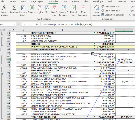
*The icon means that the selected cell is referenced by a cell on another worksheet or workbook e.g. using the VLOOKUP formula in this case from the Adjustments sheet.

Step 4 : For Trace Dependents a blue tracer arrow points to another cell that depends on the cell.

*In the example above, cell E76 has several dependents which use its value to calculate subtotal and total sum amounts in cells E89, E112, E128, and E129 on the Group & Ungroup – 2 tab.

I hope that helps. Please leave a comment below with any questions or suggestions. Thank you!

[commercecurve]

Sorting function in Microsoft Excel

What is Sorting function in Microsoft Excel?

When the volume of data is humongous, sorting of data becomes essential. This helps in presentation of information in user friendly manner. Sorting can be done in multiple ways, ascending, descending, alphabetical, color, font and in numerous other ways.

In this post I will explain how to use sorting function in an Excel spreadsheet with the help of following example:

How to properly sort the data in Microsoft Excel?

Practical Application of Sorting Function

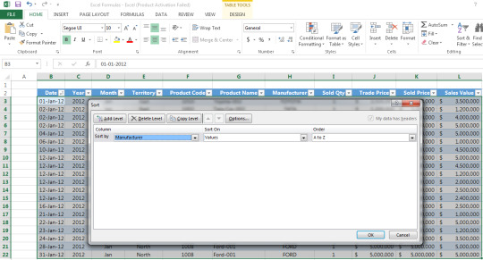
Example 1 – Suppose you are a trader of manufactured cars and want to sort the sales data as given in the table below according to the alphabetic sequence of name of manufacturers, following steps would be required to be followed

Step 1: Select the data table

Step 2: Go to Home > Sort & Filter > Custom sort

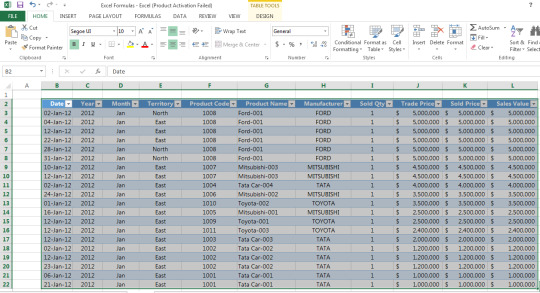
Step 3: Using the example table below, sort column data according to Manufacturer, sort on Cell Values and set the Order as A to Z

* Using the “Add Level” button you can also add an additional level of filtering (e.g. by product name)

Step 4: Press ok and your data will be sorted accordingly

How to sort data from smallest to largest in Microsoft Excel?

Further, in case you want to sort the same data from smallest to largest numbers in terms of sales value, following conditions would be required to be selected:

Step 1: Sort column according to Sales Value and set the Order as Largest to Smallest.

Step 2: Press ok and your data will be sorted accordingly

I hope that helps. Please leave a comment below with any questions or suggestions. Thank you!

[commercecurve]

What is Data Validation in Excel

What is Data Validation in Excel:

Data validation is the function in Excel that is used to control what data can be input in a particular cell or range of cells.

When inputting the data, data validation can display a message for the user regarding what type/kind of data can be input.

It also stops the user from inputting the data other than that allowed by the data validation function and can give an error message when invalid data is entered.

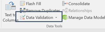
Where to find Data Validation in Excel:

Go to:

Data > Data Tools > Data Validatoin

1. Data

2. Data Tools

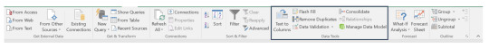
3. Data Validation

Data Validation Criteria:

Data validation function in excel can be used to limit data input to following criteria:

Any value: This is the default value set by Excel for Data Validation, if there are no Data Validation restrictions, we can enter any value in any cell of excel spreadsheet.

Whole number: Allowing only to input a whole number in the cell

Decimal: Allowing only decimals in the cell

List: Allowing the input of data from a pre-defined list.

Date: Allowing input of data in date format only.

Time: Allowing input of data in time format only.

Text length: restricting the number of text characters, that can be input in the cell.

Custom: Specifying a custom formula to restrict the input of data according to that formula only.

How to use Data Validation function in Excel:

Let’s take an example here, where we are inputting expenses relating to a project in a table in Excel, and we want that our cells in the table only allow a particular type of data to be input in the cells to avoid any mistakes.

We have following fields in the table to populate.

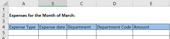
We can use different data criteria in these columns to allow particular set of data to be input in these, by using the data validation function.

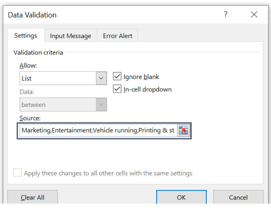
How to use restrict data from dropdown list only using data validation:

Continuing with the above example, we want our “Expense Type” column to be populated using a dropdown list of following categories:

Marketing

Entertainment

Vehicle running

Printing & Stationery

How to add a dropdown list using data validation function in Excel:?

Step 1. Select the cell or range of cells where we want the data validation function to allow only drop down list.

Step 2. Go to data validation function.

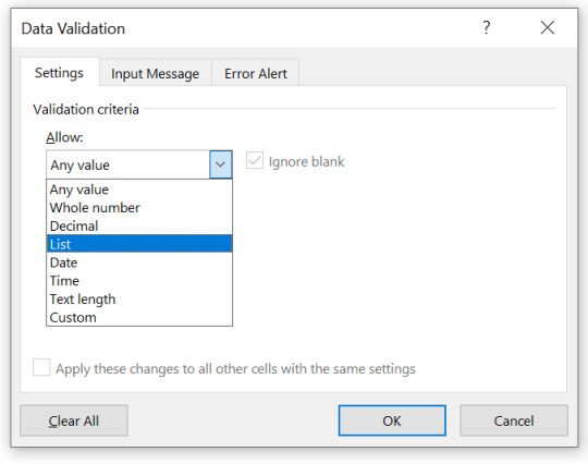
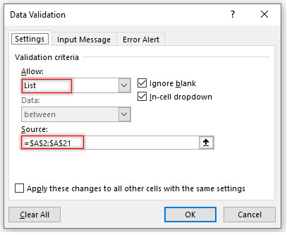
Step 3. In validation criteria, select “List”.

Step 4. In source field, either write down the list by separating each item in list using coma.

Or, you can put your list somewhere in excel, and put the range of cells containing list in the source field.

Step 5. Click OK to complete the data validation function.

How to use data validation function to customize date entry in excel?

Continuing with our sample table from the table above, in the column “expense date” we want only dates relating to the month of March, 2020 to be entered. We can use data validation function in excel to restrict that only the dates between March 01, to March 31 can be entered in this column.

Step 1. Select the cell or range of cells where we want data validation function.

Step 2. Go to data validation function.

Step 3. In validation criteria, in “Allow field” select “Date”.

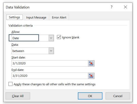
Step 4. In the “Data” field, select “between”.

Step 5: Give the desired start and end dates, which in our case are March 1, 2020 & March 31, 2020 respectively.

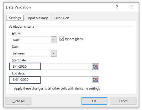
Step 6: Click OK to complete the data validation function for date restriction.

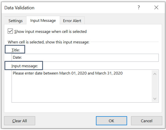
How to add an input message using data validation:?

Data validation function allows to add an input message on the cell or range of cells where data validation function has been applied, to give the user a guidance on what type/kind of data can be entered.

Step 1. Go to data validation.

Step 2. Go to tab “input message”.

Step 3. Add Title and the message you want to display when the cell or range of cells is selected.

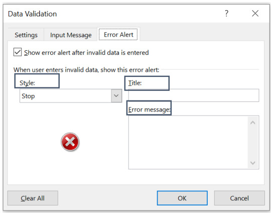
How to add an error message in data validation function:

Data validation function in excel allows to add an error alert to be displayed, if invalid data is entered in the cell or range of cells.

Step 1. Go to data validation function in excel.

Step 2. Go to the tab “Error Alert”.

Step 3. Select style, title and the error you want to be displayed once the invalid data is entered into.

[commercecurve]

Scenario Manager in Excel

What is Scenario Manager in Excel

Scenario Manager function in excel can be used for making different scenario such as good, bad, moderate, based on certain range of output/input which impact the ultimate outcome.

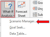
Where to find Scenario Manager in Excel:

Go to:

Data>Forecast>What-If Analysis>Scenario Manager

1. Data

2. Forecast

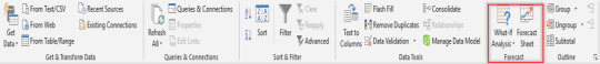
3. What-If Analysis – Scenrario Manager

How to use Scenario Manager Function in Excel:

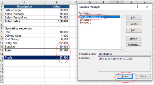
Let’s take an example of XYZ company to understand$ the different fields of Scenario Manager Function. Total profit of the XYZ company for the month is 67,500. The company want to see the impact of increase/decrease in cost of supplies and utility bills on its monthly profit. Scenario Manager Function of Excel helps XYZ Company to see what the monthly profit of the company will be if values of supplies and utility bills change.

Step 1: Create a table in excel showing monthly Profit & Loss of the company.

Step 2: By clicking on Scenario Manager Following dialog box will open:

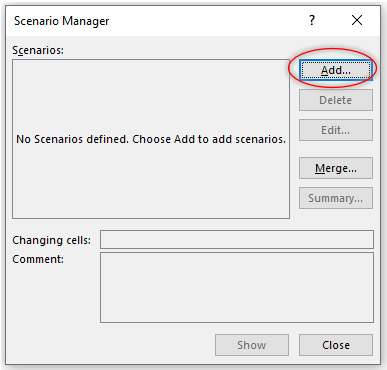
Step 3: Now add a new scenario by clicking on Add button. Following dialog box will open.

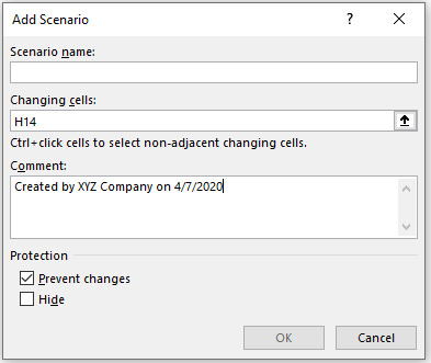
Type the Scenario name, in our example we are going to name it “Monthly Profit & Loss”:

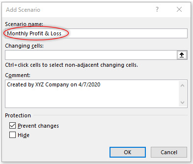
Changing cells field will allow the cells which hold our values which we want to change. As XYZ wants to see the impact of supplies and utility bills cost on its profits. Therefore, select cells that contain value of supplies and utility bills.

Click OK and change the values of supplies and utility bills as per our example

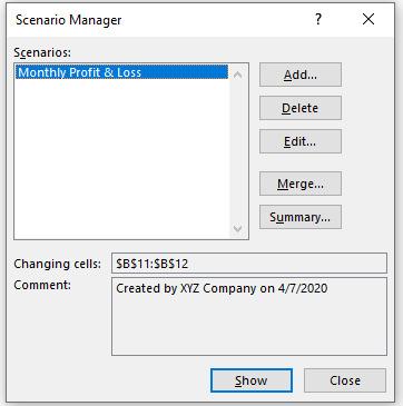
Go back to Scenario Manager window by clicking OK. Now the Scenario Manager dialog box will look like:

The first scenario has been created. Now create the scenario 1 and scenario 2 following the above steps which depicts the changes in the given scenario.

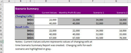
In case of scenario 1 change the values of utility bills and supplies to 34,000 & 52,000 respectively.

In case of scenario 2 change the values of utility bills and supplies to 18,000 & 35,000 respectively.

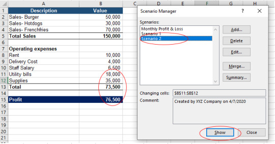
Now we have Monthly Profit & Loss, Scenario 1 and Scenario 2. Select each scenario one by one, click show, the Scenario Manger function of the Excel will calculate the monthly profit with each Scenario.

Check that by selecting scenario 2, Scenario Manager Function will calculate monthly profit & loss depicting the changed values of utility bills and supplies. You may notice that with Scenario Manager function there is no need to put values each time to see the impact of change values.

Check that by selecting scenario 1, Scenario Manager Function will calculate monthly profit & loss depicting the changed values of utility bills and supplies. You may notice that with Scenario Manager function there is no need to put values each time to see the impact of change values.

Check that by selecting scenario 2, Scenario Manager Function will calculate monthly profit & loss depicting the changed values of utility bills and supplies. You may notice that with Scenario Manager function there is no need to put values each time to see the impact of change values

How to Create Summary Report in Excel

1. Data>Forecast>What-If Analysis>Scenario Manager>Summary

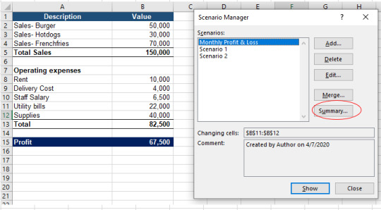
Click Summary and following window will open:

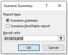
By clicking OK, a Summary will be created in new Excel sheet. Check how Scenario Manager Function has created a summary showing the change under each case and the impact of that change on the profits of the XYZ Company.

[commercecurve]

Text to column function in Microsoft Excel

What is Text to Column function in Microsoft Excel?

Text to column function is used to split cell contents into multiple columns depending on the criteria set. Exported data from a system contains a mix of data attributes. You need the data to be split up so that you can only the relevant part of it.

In this post I will explain you how to use text to column function in an Excel spreadsheet with the help of following example:

Practical example of Text to column function

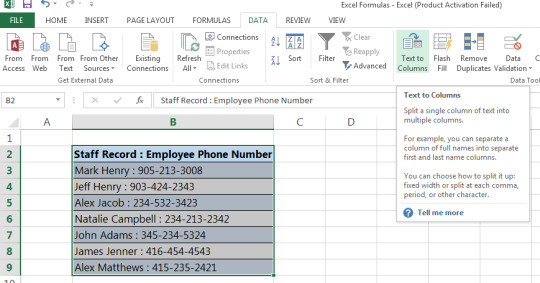
The HR Analyst received data exported from the company’s HR database containing employee name and phone number in the same cell. The HR Analyst needs to make a list of the employee name in a column separate from their phone number:

Step 1: Highlight data in table, Go to Data tab and click on Text to Columns

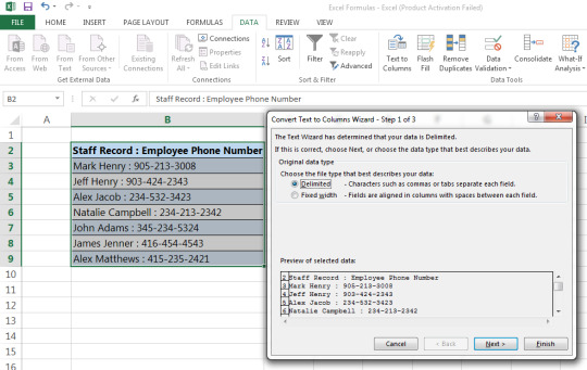
Step 2: Select delimited if you’d like to separate data that has characters or a space between the data

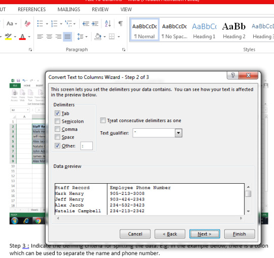
Step 3: Indicate the defining criteria for splitting the data. E.g. in the example below, there is a colon which can be used to separate the name and phone number.

Step 4: The data will split into two cells as is required

I hope that helps. Please leave a comment below with any questions or suggestions. Thank you!

[commercecurve]

Remove Duplicates Function in Microsoft Excel

What is Remove Duplicates Function in Microsoft Excel?

Remove duplicates function is used to remove duplicate values from a series of data in a table. This is a commonly used function if you need to find only unique values of a characteristic of data within a table.

If a data table contains an abundance of data and you want to make a list of the unique items only then this formula is often handy.

In this post I will explain how to use remove duplicates function in an excel spreadsheet with the help of following example:

What are the steps to perform a Remove Duplicates Function in Microsoft Excel?

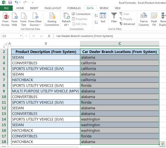
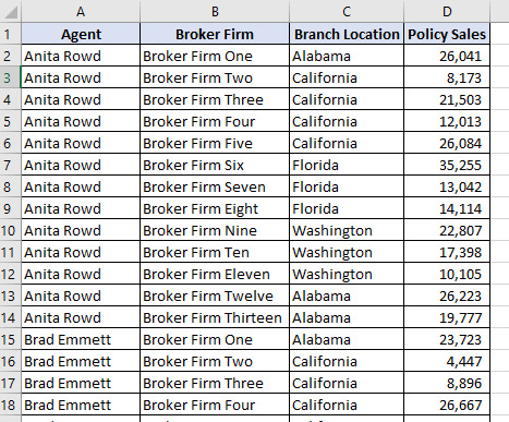
Suppose the Financial Analyst received data exported from the company’s ERP system and it contained product information and the product descriptions. The Financial Analyst wants to make a list of all the unique car dealer branch locations.

Step 1: Select the column in the table for car dealer branch locations.

Step 2: Go to data tab and click on remove duplicates

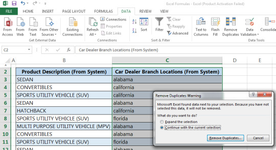
Step 3: After clicking on “Remove Duplicates” and you will get the result of removing duplicate values from the car dealer branch location column as shown below.

I hope that helps. Please leave a comment below with any questions or suggestions. Thank you!

[commercecurve]

Name Manager in Excel

What is Name Manager Function in Excel?

Name Manager function of excel is used to add, edit, delete and find the name of a particular cell, cell range, formulas, tables etc. This function increases the understandability of the formulas by giving the cell reference a particular name.

Where to find Name Manager in Excel:

Go to: Formulas>Defined Names>Name Manager

How to use Name Manager Function in Excel?

Example 1

Let’s understand how to use Name Manager Function. Suppose we want to name cell range A1:A10 as “Google”. We need to fill Name and Refers to fields of Name Manager as follows:

Name: Google

Refers to: A1:A10

Step 1:

Click on Name Manager and following dialog box will open:

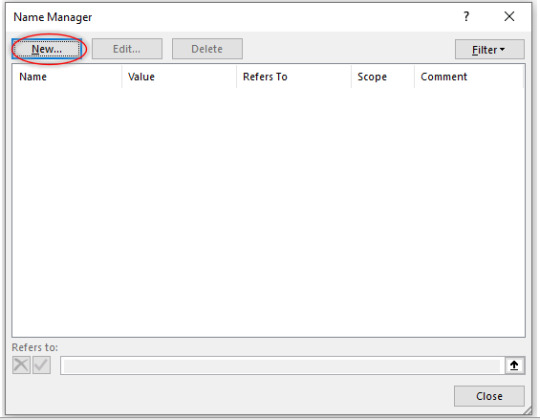
Step 2: Click New button and following dialog box will open:

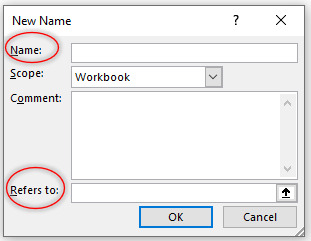
Name: allows us to specify the readable and meaning full name of a cell, cell range.

Scope: determines whether specified name will be local to work sheet or apply to the whole workbook.

Comment: allows us to write any additional note/information.

Refers to: specify the range of cell which we want to name.

Step 3: Type Google and select range of cells you want to name in Name and Refers to fields respectively. The window will look like:

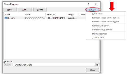
Click Ok and window will look like this:

Now you can see that Edit, Delete and Filter buttons are also active. If you want to edit the name Google first select the name Google and click Edit button and change the name.>/p>

If you want to delete the name Google just select that name and click Delete. Option to Delete can be used to delete different name at same time, select one name hold ctrl/shift button of your keyboard and select names you want to delete. Release the ctrl/shift key and click delete button.

Similarly, you can filter your name range by using the Filter button. Click on Filter button and the following options will be available to you.

Example 2

Let’s take another example to see that how Name Manager function of Excel increases the understandability of any formula.

Suppose ABC Company produces four products and its sales for the month of January, February and March is as follows:

The company wants its sale range to be name as per product because this will enhance the understandability of the formula.

Let’s check how Name Manager helps in achieving that objective of the company. Add the products name and cell range you want to sum up using the Name Manager Function as described above. The window will look alike.

See that after using the Name Manage Function you may obtain the total sales for the month of January, February and March by just putting the name of the product.

You may notice how Name Manager gives a cell and cell range a meaningful and readable name instead of cell reference. Now anywhere on the sheet or the workbook, depending upon the scope we have chosen while giving the range a name, we can just use the range name “Alpha” in our formula to reference January through March sales.

[commercecurve]

INDIRECT Function in Excel

What is INDIRECT Function in Excel?

INDIRECT function of Excel is used to give reference to the cell, cell range, any named range, work sheets or workbook. In simple words INDIRECT function is used to refer the cells, cell range of different work sheets or workbook in any formula and converts the text string into a valid cell reference. In this way, cell reference in a formula can be changed easily without changing the formula itself.

This function is useful when data set is spread across multiple work sheets or workbooks and we want to use this data on another work sheet or workbook.

Another advantage of INDIRECT function is that any indirect reference created through this function does not change when new rows/columns are added or deleted in a work sheet.

Where to find INDIRECT Function in Excel?

Formulas>Lookup & Reference>INDIRECT

How to use INDIRECT Function?

Let us understand how to use INDIRECT function in Excel.

Example 1

Suppose we have data of different football leagues and number of matches played by them in the below table:

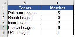
and we want to convert the text in Teams column with valid cell reference. Let us check how INDIRECT function helps us in doing this.

Step 1: Select the cell in which you want to insert INDIRECT function. Open the INDIRECT function as explained above and following dialog box will appear.

Ref_text: is a cell reference or text string (or both) or named range.

A1: It is optional and a logical value that specifies the type of reference in Ref_text field.

A1-style       = TRUE or omitted

R1C1-style   = FALSE

A1-style is the reference type of Excel which refers to column followed by row number. For example, C5 refers to the cell at intersection of column C and row 5. Excel normally follows this reference style.

R1C1-style is the reference type of Excel which refers to row followed by column number. For example, R2C3 means row 2 and column 3 i.e. C2. In order to use this style, you must go to File>Options>Formulas>R1C1 and then check the R1C1 box.

As A1 is the usual reference style of the Excel we will use A1 in this tutorial.

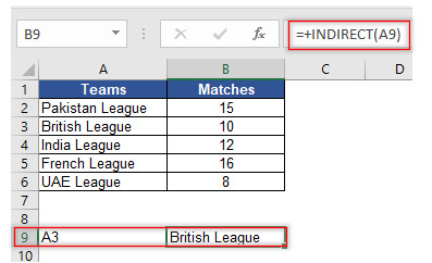
Step 2: Select A9 in Ref_text field which is cell reference of A3 (which is again cell reference of our text string British League). Leave A1 field blank as we do not want to change our cell referencing style.

You may notice that by putting A3 (the cell reference containing British League), INDIRECT function converts text string “British League” into valid cell reference.

Example 2

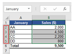
Let us take another example. We have three months sales data of different products and we want to use INDIRECT Function to get the sum of all its’ products sold for the month of January/February/March because INDIRECT reference created does not change with any addition/deletion of rows/columns whereas normal sum function does not include the cell range which are added after initial specified sum range. Let’s understand how the INDIRECT function helps in achieving that objective.

Step 1: Create name range for the all months (Formulas>Name Manager). Select the cell where you want to insert combine Sum & INDIRECT function.

You may notice that in case of INDIRECT function you have to only insert the cell reference of “January” and this function converts text string “January” into a valid reference B1.

Example 3

Suppose Winter Limited sales data for all the three months is spread across in three different work sheets and it wants to prepare a summary sheet showing sum of its three months sales. It wants to use combine Sum and INDIRECT function for this purpose as well. Let’s see how INDIRECT might be used in this situation.

Step 1 Cell range of the data set should be same for all the three separate sheets viz. January, February & March. In this example cell range B2:B5 contains the sales values for the month of January, February & March (in separate worksheet).

Step 2 Select the cell where you want to Sum the January sales using INDIRECT function.

Step 3 Insert the formula as shown below:

You may check that INDIRECT function converts the text January into a valid cell reference A2. Similarly, you can get the total for the month of February & March by just replacing A2 with A3 & A4 respectively in the above formula and the INDIRECT function gives you the total sales for these months.

[commercecurve]

Conditional Formatting function in Microsoft Excel

What is Conditional Formatting in Microsoft Excel? How is Conditional formatting used in a project?

Conditional formatting in Excel enables you to highlight cells with a certain color depending on the cell’s value. This is a beneficial function when you want to draw attention to data that meets certain value criteria.

In this post I will explain you how to use conditional formatting function can be explained with the help of following example:

Practical applications of Conditional formatting function

Example 1

Suppose you have a sales report for January 2017, and would like to highlight the sales that are less than 4,000,000.

Step 1: Select the row or column that you want to format

Step 2: Go to Home tab > Conditional formatting > Highlight cells rules > Less than

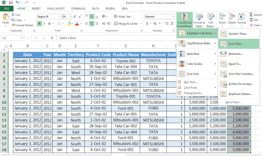
Step 3: Insert value on format cell that are LESS THAN, and set your condition (e.g. Light Red Fill with Dark Red Text

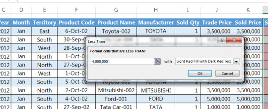
Step 4: Then click OK

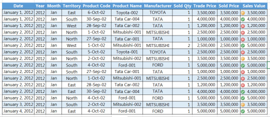
Example 2

Suppose you have a sales report for January 2017 and would like to indicate beside the sales values certain symbols depending on whether they are at satisfactory level or not based on the following conditions:

>$4,000,000, denote with checkmark sign,

<$4,000,000 and >$3,000,000, denote with an exclamation mark sign,

<$3,000,000 denote with a cross mark

Step 1: Select the row or column that you want to format

Step 2: Go to Home tab > Conditional formatting > Icon sets > More rules

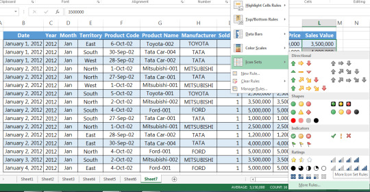
Step 4: Modify the rule based on your preferences. In our example, we have selected the respected signs as were required in the report and have giving the numeric conditions accordingly

Step 5: After selecting the required signs and mentioning the numeric conditions, click OK

I hope that helps. Please leave a comment below with any questions or suggestions. Thank you!

[commercecurve]

Dependable Drop-Down Function in Excel

What is Dependable Drop-Down Function in Excel?

Dependable drop-down function is an advanced function of data validation that allows us to create simple drop-down lists. With the help of dependable drop-down function, we can create drop-down lists for more than one cell, in such a way that items in dependent list change as we change the item in the drop-down list. This is useful when working with database with lots of categories & subcategories and makes data entry easier by just picking up the item from parent drop-down list and then dependent drop-down list.

Where to find Dependable Drop-Down Function in Excel?

Go to:

Data>Data tools>Data Validation>Settings

How to use Dependable Drop-Down Function?

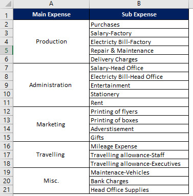
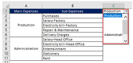
Let us take an example to understand Dependable Drop-Down function. Suppose Zee Limited has different categories & subcategories of expenses. It wants to create a drop-down list for its main category of expenses and later on, on the basis of the main category of expenses, a drop-down list of sub category of expenses so that data can be entered easily, efficiently and without any error. We can use drop-down function to arrange data in the way Zee Limited wanted.

Step 1: Select cell where you want the parent drop-down list. Open Data validation and following dialog box will open:

Allow: refers to different sources for creating the drop-down list.

Data: allows different criteria for drop-down list depending upon your selection in Allow field.

Source: allows you to select the cell range to be included in drop-down list.

Step 2: In Allow field select List, in Source field specify the cell range that contains the main expenses.

Click Ok and parent drop-down list will be created.

Step 3: Create name range for all the main expenses. (Formulas>Name Manager) or using short key ctrl+f3. After creating name range for all the main expenses:

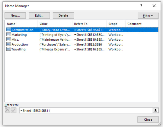
Step 4: Select the cell where you want to create dependable drop-down list. Open Data Validation and repeat the steps as explained above, except now in Source field type =INDIRECT(D2). INDIRECT function of Excel gives name range of main expenses and their sub expenses a valid reference and enable us to use this reference in creating dependable drop-down list. Please note that D2 is the cell location of parent drop-down list. The window will look like:

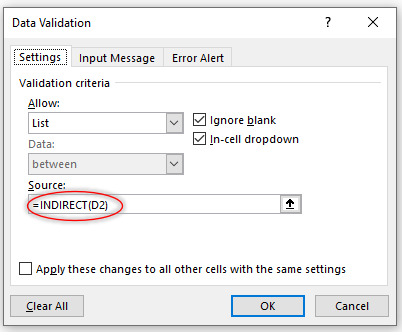
Click Ok and check the outcome:

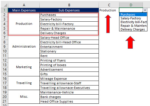
Now you have to select the main expense from parent drop-down list and dependable drop-down list will be automatically update.

You may notice that by using this function many data with different categories can be entered very efficiently and with any error.

[commercecurve]

Advanced Filtering in Excel

What is Advanced Filter Function in Excel?

Advanced Filter function of Excel is used to filter the data, when criteria to filter the data is complex. By creating a criterion through Advanced Filter function, you can extract unique data from large data base. This function is different from regular filter function of Excel which is accessible in just one click. Contrary to regular filter function of Excel, Advanced Filter function can extract the data to new location as well.

Where to find Advanced Filter Function in Excel?

Go to: Data>Sort & Filter>Advanced

You may use Keyboard shortcut ALT+a+q to open this function.;

How to use Advanced Filter Function?

Example 1

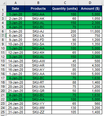
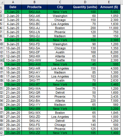
Let’s understand how to use Advanced Filter Function. Suppose we have sales data of Tee Limited for the month of January, 2020. You may notice duplication of products SKU-AA, SKU-AL & SKU BC in data table given below while entering the data. Tee Limited wants to remove the duplications without changing the original data base. Through Advanced Filter Function we can extract unique data i.e. any duplication will be removed and can also place that unique data on some new location whilst keeping our original data unchanged. Let’s understand how Advanced Filter Function helps in achieving this objective.

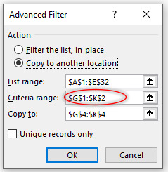
Step 1 Click the Advanced button as shown above and following dialog box will open:

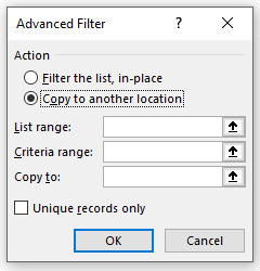
Action: This refers to the location where you can save the filtered data.

List range: This refers to the data base from where you want to filter unique data.

Criteria range: This refers to our constructed criteria for extraction/filtration of data.

Copy to: This refers to cell address where you can get the filtered data.

Check unique records only.

Please note that there should be no blank rows in your data base and also select header while selecting the List range as Advanced Filter Function consider the first cell as header.

Step 2 Fill in the above dialog box:

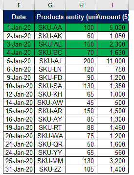
Check that how Advanced Filter Function has filter out unique data by removing the duplication.

Example 2

Using AND criteria

Let’s move one step ahead and create a criterion for filtering the complex data base. Suppose Tee Limited sells its products in different cities of USA and wants to know its sales in New York city and greater than $2,000.

Let’s understand how Advanced Filter Function helps Tee Limited in achieving this objective.

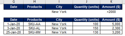
Step 1 Copy the header and paste on another place in the work sheet.

Step 2 As we want to see sales greater than $ 2,000 in New York city therefore enter in new cell New York & >2000 below the City and Amount respectively.

Step 3 Now fill in the fields of Advanced filter function as explained above. Give criteria range by selecting the entire cell range as shown above. The window will look like.

See how Advanced Filter Function filter out the sales greater than $ 2,000 in New York city.

Example 3

Using OR criteria

Let’s take same example to understand the OR criteria. Now Tee limited wants to see its sales either in Washington or Phoenix. Repeat the steps which you have performed in example 2 above except now criteria will be specified in the same column.

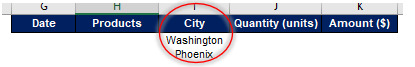
The end result will be as follows:

See how Advanced Filter Function of Excel makes the filtration of large data base on given criteria and identification of any duplication/error while entering the data in just few minutes thus saving lot of time.

[commercecurve]

Automate Database Reports with Record Macro Function in Excel

How to use Record Macro Function in Excel to Automate Database Reports?

Automation of Database Reports with the Record Macro Function is useful when you export database reports in excel for your everyday reporting purposes. For example, preparing inventory reports or conducting sales analysis and there is a certain set of repeated steps that you must always follow to prepare the report. If you have identified the steps that are repeated all the time, you can be easily automate them to save time.

In this post, I will explain to you how to use the Record Macro Function in Excel to Automate Database Reports.

Practical applications of Automating Database Reports with Record Macro Function.

Example

Suppose you have a sales database report and you would like to automate it so that you can calculate the total units sold by each sales representative.

Step 1: Save your Excel file as Macro Enabled Workbook.

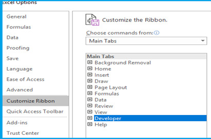
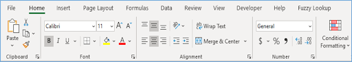
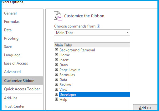
Step 2: Enable Developer Tab in your workbook. Go to File>Options>Customize Ribbon>From Drop Down Select Main Tab>Developer Tab>Add>OK

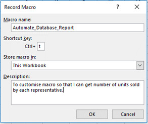
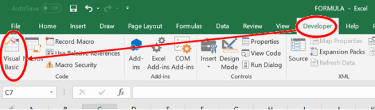
Step 3: From the Developer Tab, click Record Macro and this will prompt you to a Macro Window.

Step 4. (i) Select a name for the Macro. Please note that any spaces in the name should be filled with underscore “_” as it does not allow spaces.

   (ii) Select a short cut key (optional).

   (iii) Option to store the macro in either the same workbook or elsewhere.

   (iv) You can add a description so that you can remember the reason why the macro was created (Recommended).

Step 5: Once you press “OK”, the macro will start recording automatically.

Step 6. You can now proceed to carry out the activity on your database workbook the same way you want it to be automated. In the example above, we will select column C and paste it in Column J. Please make sure not to use any shortcut keys as this can confuse the VBA editor.

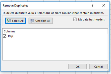
Step 7. Select Column J and go to Data Tab > Remove duplicates. A remove duplicates dialogue box will appear, press OK to get unique representative names.

Step 8: Now Select Cell K1 and name it “Total Units sold”. Below it, type the SUM IF formulae “=SUMIF(C:C,J2,E:E)”. Drag and paste the formulae against all the empty cell. Please make sure not to paste in on the entire column as it will make the worksheet heavy.

Step 9. Go to Developer Tab>Stop Recording. This will stop recording the macro and save it.

Step 10: To view how the VBA has recorded your macro, go to Developer Tab>Visual basic. This will open the VBA editor showing how the formula has been saved. Check for errors and correct them. The formula should look like provided below.

Explanation of the VBA Code

The VBA code shown above is further explained below for the users to understand so that they can customize it themselves if they want the result to be different as per their needs.

   ActiveCell.Offset(0, 2).Columns(“A:A”).EntireColumn.Select

The first layer is simply the Offset function which directs excel to move from one cell to the other based on a specific row and column number. In the beginning, the pre-defined excel cell will be the Cell A1. So, from the Syntax, we are telling excel to move zero rows and two columns forward from the cell A1. Once excel moves to cell C1, we are asking it to select the entire column.

   Selection.Copy

The second layer is instructing excel to copy the selected column.

   ActiveCell.Offset(0, 7).Range(“A1”).Select

In the third layer, we are again using the offset function. Please note, that in this case, the Active Cell has now changed to C1 because of previous selection. After moving seven columns forward from the cell, the new active cell will be the cell J1.

   ActiveSheet.Paste

The fourth layer is instructing excel to paste the copied column on the new active cell.

   ActiveSheet.Range(“J:J”).RemoveDuplicates Columns:=1, Header:=xlYes

The fifth layer is the remove duplicates function. We are simply selecting the entire Column J and removing the duplicate values. The Syntax is also defining that the data for remove duplicates is in one column and it contains a header as well.

  ActiveCell.Offset(0, 1).Range(“A1”).Select

The sixth layer is simply the offset function to select cell K1.

   ActiveCell.FormulaR1C1 = “Total Units Sold”

In seventh layer, we type the header.

   ActiveCell.Offset(1, 0).Range(“A1”).Select

In the eight layer, we are instructing excel to move one row downwards.

   ActiveCell.FormulaR1C1 = “=SUMIF(C[-8],RC[-1],C[-6])”

In the ninth layer, we can see that now the active cell is K2. The code simply enters the SUM IF  formulae where it selects the Column C having the representative names and Column E having the total units sold. The negative numbers represent corresponding column distance from selected cell. Leftward or upward cell movements are represented by a negative sign.

   ActiveCell.Select

   Selection.Copy

   ActiveCell.Offset(1, 0).Range(“A1:A10”).Select

   Selection.PasteSpecial Paste:=xlPasteAll, Operation:=xlNone, SkipBlanks:= _ False, Transpose:=False

The Last part of the VBA code is simply copying the SUM IF formulae to the rest of the representative names to give the result next to each representative name.

Now that you understand how the Record Macro works in Microsoft Excel and stores the VBA Code to automate database reports, you can also customize it as per your needs.

I hope that helps. Please leave a comment below with any questions or suggestions. For more in-depth Excel training, checkout our Ultimate Excel Training Course here. Thank you!

[commercecurve]

Automate Database Reports with VBA Code in Excel

How to use VBA code in Excel to Automate Database Reports?

Automation of Database Reports with VBA code is useful when you export database reports in excel for your everyday reporting purposes, for example, preparing inventory reports or conducting sales analysis and there is a certain set of repeated steps that you have to always follow to prepare the report. If you have identified the steps that are repeated all the time, you can be easily automate them to save time.

In this post, I will explain to you how to use VBA Code in Macro, provided in the following example, and use it to Automate Database Reports.

Practical applications of Automating Database Reports with VBA

Example

Suppose you have a sales database report and you want to automate it so that you can extract the total units sold by each sales representative.

Step 1: Save your Excel file as Macro Enabled Workbook.

Step 2: Enable Developer Tab in your workbook. Go to File>Options>Customize Ribbon>From Drop Down Select Main Tab>Developer Tab>Add>OK

Step 3: Go to Developer Tab>Visual Basic

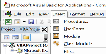
Step 4: Go to Insert Tab>Module.

Step 5: Copy the VBA code below and Paste it on Macro Visual Basic Module.

Step 6: Press F5 or the Play button to run the task and generate report as shown in the example above.

Explanation of the VBA Code

The VBA code shown above is further explained below for the users to understand so that they can customize it themselves if they want the result to be different as per their needs.

   ActiveCell.Offset(0, 2).Columns(“A:A”).EntireColumn.Select

The first layer is simply the Offset function which directs excel to move from one cell to the other based on a specific row and column number. In the beginning, the pre-defined excel cell will be the Cell A1. So, from the Syntax, we are telling excel to move zero rows and two columns forward from the cell A1. Once excel moves to cell C1, we are asking it to select the entire column.

   Selection.Copy

The second layer is instructing excel to copy the selected column.

   ActiveCell.Offset(0, 7).Range(“A1”).Select

In the third layer, we are again using the offset function. Please note, that in this case, the Active Cell has now changed to C1 because of previous selection. After moving seven columns forward from the cell, the new active cell will be the cell J1.

   ActiveSheet.Paste

The fourth layer is instructing excel to paste the copied column on the new active cell.

   ActiveSheet.Range(“J:J”).RemoveDuplicates Columns:=1, Header:=xlYes

The fifth layer is the remove duplicates function. We are simply selecting the entire Column J and removing the duplicate values. The Syntax is also defining that the data for remove duplicates is in one column and it contains a header as well.

  ActiveCell.Offset(0, 1).Range(“A1”).Select

The sixth layer is simply the offset function to select cell K1.

   ActiveCell.FormulaR1C1 = “Total Units Sold”

In seventh layer, we type the header.

   ActiveCell.Offset(1, 0).Range(“A1”).Select

In the eight layer, we are instructing excel to move one row downwards.

   ActiveCell.FormulaR1C1 = “=SUMIF(C[-8],RC[-1],C[-6])”

In the ninth layer, we can see that now the active cell is K2. The code simply enters the SUM IF  formulae where it selects the Column C having the representative names and Column E having the total units sold. The negative numbers represent corresponding column distance from selected cell. Leftward or upward cell movements are represented by a negative sign.

   ActiveCell.Select

   Selection.Copy

   ActiveCell.Offset(1, 0).Range(“A1:A10”).Select

   Selection.PasteSpecial Paste:=xlPasteAll, Operation:=xlNone, SkipBlanks:= _

       False, Transpose:=False

The Last part of the code is simply copying the SUM IF formulae to the rest of the representative names to give the result next to each representative name.

Now that you understand how the VBA Code works to automate database reports, you can also customize it as per your needs.

I hope that helps. Please leave a comment below with any questions or suggestions. For more in-depth Excel training, checkout our Ultimate Excel Training Course here. Thank you!

[commercecurve]

Fuzzy Lookup Function in Excel

What is Fuzzy Lookup Function in Excel?

Fuzzy Lookup Function is used to lookup two tables that have similar data but with minor differences, such as a spelling error. All the lookup functions in Excel, perform only when there is exact match between two sets of Data. Often, people make mistakes while preparing data such as instead of using the database code or naming convention, they manually type the name which results in slight difference between the name store in the database. To correct the data error, you must go through a cumbersome process of looking at each mistake and correcting it. We can easily compare data that has minor changes by the help of Fuzzy Lookup Function in Excel.

It comes in the form of external add-in which is available on Microsoft Website and it can be downloaded for the link “https://www.microsoft.com/en-ca/download/details.aspx?id=15011” .

Practical applications of Fuzzy Lookup Function in Excel

Example

We are using a sample database file that contains item code and item names. We want to upload the revision of prices to our Database and we have prices in a different sheet but the item names on that sheet have some spelling error due to which the lookup functions will return an error. Therefore, we will use the Fuzzy Lookup Function to compare the two tables side by side.

Step 1: Go to the Link: https://www.microsoft.com/en-ca/download/details.aspx?id=15011 and download the Fuzzy Lookup Add-in.

Step 2:  An installation window will open, install the add-in from there. When you open the next instance of Microsoft Excel, the Fuzzy Lookup Tab will automatically appear in the Main Tabs.

Step 3: Copy your Database item names and price list item names in separate sheets in Column A. Then convert both lists in separate worksheets into Tables. To convert the lists into tables, Go to Insert Tab > Table. A create table window will appear. Click Ok to convert the list into Table. The reason for doing this is to instruct Excel to perform the Fuzzy Lookup Function on the table rather than on a particular cell.

Step 4: Navigate to Fuzzy Lookup from the Fuzzy Lookup Tab. A window will appear to your right. Read through it and select the following according to your need. (i) Select number of matches as one if you want the match to return the closest match. Otherwise you can change this for multiple matches. (ii) Select the similarity threshold according to the level of accuracy you want the data to be in. It is a good practice to use sensitivity of 0.9-1.0 as this will give more accurate results.

Step 5: The result will be as shown below. The Fuzzy Lookup Function will compare both Tables and show the Similarity threshold between both list items. You can now use this as a reference point for your workings. To get the prices against the database item names, simply use the VLOOKUP function on the database item names and copy the corresponding price list item names from the Fuzzy Lookup comparison sheet. Then use the price list item names that were copied with the VLOOKUP function and again use it to VLOOKUP the Prices from the Price List.

Now that you understand how the Fuzzy Lookup Function works, you can use it to compare any set of data that contains minor errors. You might also have data that have multiple error for the same name and for that purpose you can set the Match to more than 1 as explained in Part Four of Step Four. You can experiment and work around the Fuzzy Lookup Function-in to get a better idea of how it can be suited to your needs.

I hope that helps. Please leave a comment below with any questions or suggestions. For more in-depth Excel training, checkout our Ultimate Excel Training Course here. Thank you!

[commercecurve]

Remove Foreign Language Characters with VBA Code in Excel

How to use the VBA Code in Excel to Remove the Foreign Language Characters?

Remove Foreign Language Characters with VBA Code is useful when you have Excel reports having both English and Foreign language text. To remove the foreign text, you must manually select each cell and remove the foreign text to be able to use the reports. This makes the whole process lengthy. We can remove the foreign text using the VBA code provided below.

In this post, I will explain to you how to use VBA Code in Macro, provided in the following example, and use it to Remove Foreign Language Characters.

Practical applications of Remove Foreign Language Characters with VBA

Example

Suppose you have a policy sales report of agents in both English and Chinese Language and you want to remove the Chinese Characters from the Excel File.

Step 1: Save your Excel file as Macro Enabled Workbook.

Step 2: Enable Developer Tab in your workbook. Go to File>Options>Customize Ribbon>From Drop Down Select Main Tab>Developer Tab>Add>OK

Step 3: Go to Developer Tab>Visual BasicStep

Step 4: Go to Insert Tab>Module.

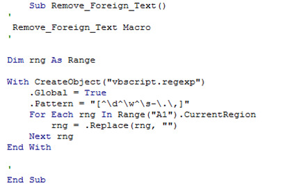
Step 5: Copy the VBA code below and Paste it on Macro Visual Basic Module.

Step 6: Press F5 or the Play button to run the task and remove the foreign language characters as shown in below.

Explanation of the VBA Code

The VBA code shown above is further explained below for the users to understand how the VBA Syntax works to remove the Foreign Language Characters.

Dim rng As Range

The first layer defines the dimensions of the values in the worksheet. The dim term refers to Dimension here. To make it simple to understand, suppose you have an excel sheet containing alphabets and numbers. If we want to select only numbers, we will set the dimension range as “Integer”. In this case, we are using the entire range and not specifying what the contents of the excel should be because we want to separate both languages so we will try to select both. This is also to ensure that if there are any numbers present both in English and foreign text, we can keep the English numbers and remove the foreign ones.

With CreateObject(“vbscript.regexp”)

The second layer is used to generate a visual basic script for regular expressions. Visual basic has a set of regular expressions stored, for example, in case of English language, it must have all the alphabets stored from A to Z in both upper case and lower-case format. It also must have numbers and punctuations. We are using With statement with Create Object. In VBA, with statements can be used to perform a series of statements on a specified object. The Object here is to run VB script for regular expressions. We will define the specific parts of the regular expressions that we want to extract in the next layers. This will help us define regular expressions of English language so that all other foreign text is removed.

   .Global = True

The third layer is the Global setting to define how the regular expression is to be processed on the worksheet, that is, whether the operation is to be processed for all the values or only on the first match. By default, it is set to False which means that when we process the code, it will only remove the first foreign character on each cell. Therefore, it must be changed to True so that it searches for all the possible values and update them.

   .Pattern = “[^\d^\w^\s-\.\,]”

The fourth layer is where we are required to define the pattern so that only the English language is detected and all else is removed. Let us look at all the patterns in the code.

The “circumflex symbol” which is usually used as mathematical exponential calculation, is used inside square brackets to look for all the other values mentioned in the square bracket. If you remove the symbol, it will remove the English Text and we will be left with the foreign one. It is necessary to have this Symbol in the code as it ensures that all the English Text is searched for.

The “back slash lower case d” symbol is used to match any single decimal digit in the range such as the number five. We will use this Syntax to find numbers accepted in the English Text.

The “back slash lower case w” symbol is used to match any alphanumeric character in the range such as the letter a. We will use this Syntax to find alphabets accepted in the English Text.

The “back slash lower case s minus” symbol is used to ignore any white spaces or tabs such as inverted commas or hyphens. We will use this Syntax to avoid any unnecessary punctuation in the text.

The “back slash lower case full stop” symbol is used to match text relating to full stop symbol. We use it to get this punctuation at the end of complete sentences.

The “back slash lower case comma” symbol is used to match text relating to comma symbol. We use it to get this punctuation in mid of sentences.

The complete Syntax means that we are instructing Excel to select all the numbers, alphabets and full stop and comma punctuation of English Text and ignore the rest.

   For Each rng In Range(“A1”).CurrentRegion

The fifth layer is instructing Excel to select all the cells containing both texts in the workbook denoted by Current Region Syntax. We are using this because we want to select these cells and then replace them just like in the Find and Replace function.

       rng = .Replace(rng, “”)

The sixth layer instructs Excel to replace the cells selected in the fifth layer with values following pattern defined in the fourth layer.

   Next rng

The seventh layer is simply instructing Excel to repeat the find and replace function until all the cells are replaced.

End With

The Last layer is to close the With Statement we started in the second layer to complete the code.

Now that we understand how the Syntax in the code works, we can use it to extract the English Language Text from Excel files containing both the English Language and the foreign language text. You can also remove the circumflex symbol in the pattern description to get the foreign language text instead of the English language.

I hope that helps. Please leave a comment below with any questions or suggestions. For more in-depth Excel training, checkout our Ultimate Excel Training Course here. Thank you!