
Don't wanna be here? Send us removal request.
Statistics
We looked inside some of the posts by dada-data-blog and here's what we found interesting.
Average Info
Notes Per Post
0
Likes Per Post
0
Reblog Per Post
0
Reply Per Post
0
Time Between Posts
7 days
Number of Posts By Type
Text
16
Last Seen Tumblr Blogs


Fun Fact
Tumblr is available in 18 languages.
Text
Machine Learning for Data Analysis: K-Means Cluster Analysis (python)
SUMMARY
K-Means Cluster Analysis is an unsupervised machine learning method that groups together observations based on the similarity (low variance) of the responses of multiple variables. These groups or clusters, which are subsets of the dataset, group together responses that have low variance within cluster and greater variance between each cluster. The goal is to have little or no overlap between the responses grouped into each cluster. Clustering can be used to determine which variables are similar enough to each other that they can be possible candidates for being combined into a single categorical variable.
For this assignment I used the variable “incomeperperson” that I’ve used in previous lessons for the target variable, as the “clustering assignment” variable to externally validate the clusters created by k-means, using an Analysis of Variance (ANOVA). I used the set of explanatory variables from the previous assignment as the “clustering” variables. These variables were scaled to have a mean of 0 and a standard deviation of 1.
I’m interested to see how clustering assignment variable incomeperperson is related to the clustering variables. In previous assignments the results have varied in terms of which variables are the best predictors of lower or higher income, however life expectancy and urbanrate are the most consistent in having a positive relationship to incomeperson, with and being predictors of higher income when their values are also high. Other variables that some tests have indicated are also positively related to higher income are internetuserate, relectricperperson and polityscore.
I wrote the original python code for this assignment using the 3 cluster model that was included in the code provided by Coursera for the assignment. But after creating the elbow plot and the ANOVO analyses, which both indicated two clusters might be enough, I also ran the analyses for two clusters which is also included below.
All variables are quantitative: Clustering Assigment Validation Variable: incomeperperson Domestic Product per capita in constant 2000 US$.
Clustering Variables used for K-Means Cluster Analysis: armedforcesrate: Armed forces personnel (% of total labor force) alcconsumption: alcohol consumption per adult femaleemployrate: female employees (% of population) hivrate: estimated HIV Prevalence % - (Ages 15-49) internetuserate: Internet users (per 100 people) relectricperperson: residential electricity consumption, per person (kWh) polityscore: Democracy score (Polity) urbanrate: urban population (% of total) lifeexpectancy: 2011 life expectancy at birth (years) employrate: total employees age 15+ (% of population) suicideper100TH: suicide per 100 000 co2emissions: cumulative CO2 emission (metric tons)
RESULTS
The 12 variables above were used in the cluster analysis with a total of 107 observations.
The training set was randomly selected from 70% of the dataset (74 observations) and the test set was the remaining 30% (33 observations).
The k-means cluster analyses was run on the training set using Euclidean distance and 1 to 9 clusters and an elbow curve was plotted for the variance in the clustering variables based on the clusters r-square values.
ELBOW METHOD to determine number of clusters

This “elbow’ plot shows that the average minimum distance (y-axis) of the observations from the cluster centroids for each of the cluster solutions decreases with the increase in the number of clusters (x-axis). The bend in the elbow at cluster 2 indicates that the curve might be leveling off which suggests that 2 clusters may provide an optimum balance of the fewest number of clusters and lowest distance between observations and assigned clusters. There is also a subtle bend at 3 and 8 clusters. 8 clusters may not be much a reduction. Since I already ran the Python code with 3 clusters I started the analysis with 3. However, since the results indicated that 2 might be more optimal and also ran the analysis with 2 variables. CANONICAL DISCRIMINANT ANALYSES to reduce clustering variables

To reduce the number of clustering variables canonical discriminant analyses was used. The two canonical variables used are linear combinations of the 12 clustering variables listed above. Additional canonical variables can be created but most of the variance in the clustering variables is accounted for in the first two canonical variables. The scatterplot graph is created by assigning the y-axis to Canonical Variable 2 and the x-axis to Canonical Variable 1. The scatterplot itself is the result of plotting both the Canonical Variable 1 and 2 for each of the observations in the training set and showing by color the k-means cluster that was assigned to each observation.
Reviewing the scatterplot it appears that there is relatively little overlap between the 2 canonical variables which suggests there is good separation among the three variables but all three are somewhat spread out which indicates less correlation among the observations and higher variance within each cluster than is ideal. It also shows that the teal and blue clusters are mostly clustered with negative values for Canonical variable 1 and the yellow cluster is mostly positive, suggesting that the two cluster might be enough to include most of the variance between observations.
COMPARISON OF CLUSTER VARIABLE MEANS by each cluster
Clustering variable means by cluster index urbanrate employrate lifeexpectancy armedforcesrate \ cluster 0 109.15 0.21 -0.88 0.21 1.45 1 114.97 0.60 -0.14 0.68 -0.18 2 101.21 -0.64 0.47 -0.92 -0.30
polityscore relectricperperson internetuserate femaleemployrate \ cluster 0 -1.13 0.06 -0.07 -1.45 1 0.69 0.59 0.83 0.07 2 -0.23 -0.59 -0.93 0.48
alcconsumption hivrate suicideper100th co2emissions cluster 0 -1.02 -0.37 -0.75 -0.20 1 0.81 -0.32 0.24 0.30 2 -0.52 0.70 -0.28 -0.20
In reviewing the means for all 12 clustering variables by cluster it looks like two clusters, Cluster 1 and 2, include most of the variable values that in past assignments (LASSO, Random Forests, Decision trees, etc.) have been the best predictors for the incomeperperson target/assignment variable, suggesting that two clusters may be more optimal than three.
In Cluster 0, armedforcesrate is the highest value for the variable in all 3 clusters, and employrate, polity score, female employment, alconsumption, hivrate, suicideper100th are at the lowest. In previous assignments most of these variables had little or no significance in predicting income levels. The exceptions were polity score and hivrate which for some models did have some prediction value. It suggests that this cluster is comprised of the values that are the least valuable in predicting incomeperperson, and could possibly be combined in Cluster 2 which includes variable values that in the past predicted lower income.
In Cluster 1, urbanrate, lifeexpectancy, polityscore, relectricperperson, internetuserate, alconsumption, suicideper100th and co2emissions have the highest values of all 3 clusters. All but alconsumption, suicideper100th and co2emissions were significant in predicting incomeperperson in at least one model in previous assignments. Since all of the variables that have been significant in predicting higher income in previous models have their highest value, it suggests that this cluster could be a predictor for observations with higher income per person.
In Cluster 2, urbanrate, lifeexpectancy, armedforcesrate, relectricperperson, internetuserate have the lowest value of all clusters. All but armedforcesrate were significant in predicting lower incomeperperson when the values of the variables were low. Hivrate has its highest values, which in a few previous models predicted income would be lower. Overall, the results for this clusters indicate it includes observations which would predict lower income per person.
ANOVA with Cluster Assignment variable: incomeperson
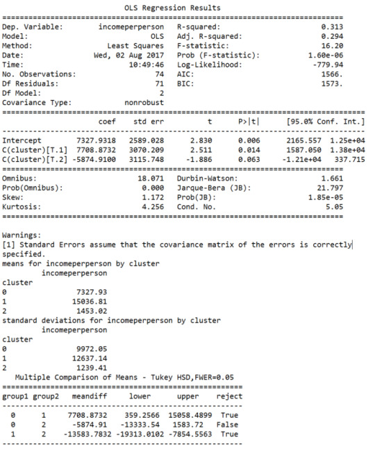
The ANOVA (Analysis of Variance) results above indicate the three clusters have significant variance : -statistic (16.20) and p value very close to 0 (1.60e-06) which suggests significant difference between clusters 0, 1 and 2.
However, the second tukey post hoc comparison test between cluster 0 and cluster 2, where “reject” is False indicates that the “null” hypothesis cannot be rejected. This result again suggests that cluster 0 may not have enough variance from cluster 2, and that two clusters may be more efficient than 3.
Below are all test result for two clusters which I think confirms that two clusters are more optimal.
RESULTS TWO CLUSTERS

The CANONICAL DISCRIMINANT ANALYSES for two clusters indicates less overlap and better separation between clusters than with three.
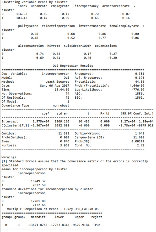
The F-statistic (44.36) and p-value (4.64e-09) for two clusters indicate greater variance between clusters than for three clusters.
CODE
# -*- coding: utf-8 -*- """ 08-1-17
@author: kbolam """
# -*- coding: utf-8 -*-
from pandas import Series, DataFrame import pandas import numpy as np import matplotlib.pylab as plt from sklearn.cross_validation import train_test_split from sklearn import preprocessing from sklearn.cluster import KMeans
""" Machine Learning for Data Analysis Random Forests """
# bug fix for display formats to avoid run time errors pandas.set_option('display.float_format', lambda x:'%.2f'%x)
data = pandas.read_csv('gapminderorig.csv')
# convert all variables to numeric format data['incomeperperson'] = pandas.to_numeric(data['incomeperperson'], errors='coerce') data['urbanrate'] = pandas.to_numeric(data['urbanrate'], errors='coerce') data['employrate'] = pandas.to_numeric(data['employrate'], errors='coerce') data['lifeexpectancy'] = pandas.to_numeric(data['lifeexpectancy'], errors='coerce') data['armedforcesrate'] = pandas.to_numeric(data['armedforcesrate'], errors='coerce') data['polityscore'] = pandas.to_numeric(data['polityscore'], errors='coerce') data['relectricperperson'] = pandas.to_numeric(data['relectricperperson'], errors='coerce') data['internetuserate'] = pandas.to_numeric(data['internetuserate'], errors='coerce') data['femaleemployrate'] = pandas.to_numeric(data['femaleemployrate'], errors='coerce') data['alcconsumption'] = pandas.to_numeric(data['alcconsumption'], errors='coerce') data['hivrate'] = pandas.to_numeric(data['hivrate'], errors='coerce') data['suicideper100th'] = pandas.to_numeric(data['suicideper100th'], errors='coerce') data['co2emissions'] = pandas.to_numeric(data['co2emissions'], errors='coerce')
data_clean=data.dropna() ''' # comment out for Cluster Assign4 #Change Target variable to binary categorical variable def incomegrp (row): if row['incomeperperson'] <= 3500: return 0 elif row['incomeperperson'] > 3500 : return 1
# added ".loc[:," to "data_clean['armedforcesgrp'] =" to get rid of copy error "Try using .loc[row_indexer,col_indexer] = value instead" # still getting error for another line but all predictors statement seem to be working with update and no more errors data_clean.loc[:,'incomegrp'] = data_clean.apply (lambda row: incomegrp (row),axis=1)
chk2 = data_clean['incomegrp'].value_counts(sort=False, dropna=False) print(chk2) ''' #select predictor variables and target variable as separate data sets #incomeperperson is sort of target variable and should not be included in cluster or clustervar cluster= data_clean[['urbanrate','employrate','lifeexpectancy','armedforcesrate', 'polityscore','relectricperperson','internetuserate','femaleemployrate','alcconsumption', 'hivrate','suicideper100th','co2emissions']]
# comment out for Cluster Assign4 #target = data_clean.incomegrp
cluster.describe()
clustervar=cluster.copy()
#need to remove incomeperperson from clustervar #clustervar['incomeperperson']=preprocessing.scale(clustervar[['incomeperperson']].astype('float64')) from sklearn.preprocessing import MinMaxScaler min_max=MinMaxScaler() clustervar['urbanrate']=preprocessing.scale(clustervar[['urbanrate']].astype('float64')) clustervar['employrate']=preprocessing.scale(clustervar[['employrate']].astype('float64')) clustervar['lifeexpectancy']=preprocessing.scale(clustervar[['lifeexpectancy']].astype('float64')) clustervar['armedforcesrate']=preprocessing.scale(clustervar[['armedforcesrate']].astype('float64')) clustervar['polityscore']=preprocessing.scale(clustervar[['polityscore']].astype('float64')) clustervar['relectricperperson']=preprocessing.scale(clustervar[['relectricperperson']].astype('float64')) clustervar['internetuserate']=preprocessing.scale(clustervar[['internetuserate']].astype('float64')) clustervar['femaleemployrate']=preprocessing.scale(clustervar[['femaleemployrate']].astype('float64')) clustervar['alcconsumption']=preprocessing.scale(clustervar[['alcconsumption']].astype('float64')) clustervar['hivrate']=preprocessing.scale(clustervar[['hivrate']].astype('float64')) clustervar['suicideper100th']=preprocessing.scale(clustervar[['suicideper100th']].astype('float64')) clustervar['co2emissions']=preprocessing.scale(clustervar[['co2emissions']].astype('float64'))
clustervar=clustervar.dropna()
clustervar.dtypes clustervar.describe()
print(type(clustervar)) #print(type(target))
# split data into train and test sets clus_train, clus_test = train_test_split(clustervar, test_size=.3, random_state=123)
# k-means cluster analysis for 1-9 clusters from scipy.spatial.distance import cdist clusters=range(1,10) meandist=[]
for k in clusters: model=KMeans(n_clusters=k) model.fit(clus_train) clusassign=model.predict(clus_train) meandist.append(sum(np.min(cdist(clus_train, model.cluster_centers_, 'euclidean'), axis=1)) / clus_train.shape[0])
""" Plot average distance from observations from the cluster centroid to use the Elbow Method to identify number of clusters to choose """ ''' plt.plot(clusters, meandist) plt.xlabel('Number of clusters') plt.ylabel('Average distance') plt.title('Selecting k with the Elbow Method') '''
# Interpret 3 cluster solution model3=KMeans(n_clusters=2) model3.fit(clus_train) clusassign=model3.predict(clus_train) # plot clusters
from sklearn.decomposition import PCA pca_2 = PCA(2) plot_columns = pca_2.fit_transform(clus_train) plt.scatter(x=plot_columns[:,0], y=plot_columns[:,1], c=model3.labels_,) plt.xlabel('Canonical variable 1') plt.ylabel('Canonical variable 2') plt.title('Scatterplot of Canonical Variables for 2 Clusters') plt.show()
""" BEGIN multiple steps to merge cluster assignment with clustering variables to examine cluster variable means by cluster """ # create a unique identifier variable from the index for the # cluster training data to merge with the cluster assignment variable clus_train.reset_index(level=0, inplace=True) # create a list that has the new index variable cluslist=list(clus_train['index']) # create a list of cluster assignments labels=list(model3.labels_) # combine index variable list with cluster assignment list into a dictionary newlist=dict(zip(cluslist, labels)) newlist # convert newlist dictionary to a dataframe newclus=DataFrame.from_dict(newlist, orient='index') newclus # rename the cluster assignment column newclus.columns = ['cluster']
# now do the same for the cluster assignment variable # create a unique identifier variable from the index for the # cluster assignment dataframe # to merge with cluster training data newclus.reset_index(level=0, inplace=True) # merge the cluster assignment dataframe with the cluster training variable dataframe # by the index variable merged_train=pandas.merge(clus_train, newclus, on='index') merged_train.head(n=100) # cluster frequencies merged_train.cluster.value_counts()
""" END multiple steps to merge cluster assignment with clustering variables to examine cluster variable means by cluster """
# FINALLY calculate clustering variable means by cluster clustergrp = merged_train.groupby('cluster').mean() print ("Clustering variable means by cluster") print(clustergrp)
# validate clusters in training data by examining cluster differences in income using ANOVA # first have to merge income with clustering variables and cluster assignment data
#may need to scale this variable income_data=data_clean['incomeperperson']
# split income data into train and test sets income_train, income_test = train_test_split(income_data, test_size=.3, random_state=123)
print ('income_train') chk1 = income_train.count() print(chk1)
print ('income_test') chk2 = income_test.count() print(chk2)
#print (income_test) income_train1=pandas.DataFrame(income_train)
#income_train1=income_train1.set_index(['incomeperperson']) income_train1.reset_index(level=0, inplace=True) #print('income_train1') #print (income_train1)
#merged_train_all=pandas.merge(income_train1, merged_train, on='incomeperperson') #THE FOLLOWING IS ORIGINAL merged_train_all=pandas.merge(income_train1, merged_train, on='index')
sub1 = merged_train_all[['incomeperperson', 'cluster']].dropna()
#sub1 = sub1.reindex(level=0, inplace=True)
import statsmodels.formula.api as smf import statsmodels.stats.multicomp as multi
incomemod = smf.ols(formula='incomeperperson ~ C(cluster)', data=sub1).fit() print (incomemod.summary())
print ('means for incomeperperson by cluster') m1= sub1.groupby('cluster').mean() print (m1)
print ('standard deviations for incomeperperson by cluster') m2= sub1.groupby('cluster').std() print (m2)
mc1 = multi.MultiComparison(sub1['incomeperperson'], sub1['cluster']) res1 = mc1.tukeyhsd() print(res1.summary())
0 notes
Text
Machine Learning for Data Analysis: LASSO Regression (python)
SUMMARY
LASSO stands for "Least Absolute Selection and Shrinkage Operator". It is a supervised machine learning method that can be useful for reducing a large set of predictor explanatory variables to a smaller set of the the most accurate predictors of the target variable. For those variables that the LASSO method determines are the least significant predictors, the coefficient is reduced to 0 and the coefficients for the variables that are the better predictors is calculated.
I added the additional explanatory variables of Carbon Dioxide Emissions and Suicide per 100th to those used for the last assignment for a total of 12 explanatory variables. All variables are from the Gapminder dataset provided by Coursera.
Target Variable: incomegrp. Gross Domestic Product per capita in constant 2000 US$. This is a binary categorial variable created from ‘incomeperperson’. 0=lower income, 1 = higher income
Predictor/Explanatory Variables:
For this assignment I used the original quantitative versions of these variables from the Gapminder dataset. I previous assignments I changed them to binary categorical variables.
armedforcesrate: Armed forces personnel (% of total labor force) alcconsumption: alcohol consumption per adult femaleemployrate: female employees (% of population) hivrate: estimated HIV Prevalence % - (Ages 15-49) internetuserate: Internet users (per 100 people) relectricperperson: residential electricity consumption, per person (kWh) polityscore: Democracy score (Polity) urbanrate: urban population (% of total) lifeexpectancy: 2011 life expectancy at birth (years) employrate: total employees age 15+ (% of population) suicideper100TH: suicide per 100 000 co2emissions: cumulative CO2 emission (metric tons)
RESULTS
The results below indicate that the following variables are the least effective predictors because their coefficient was was reduced to “0″: employrate, armedforcesrate, alcconsumption, suicideper100th, co2emissions.
The most effective predictors because they had the highest coefficent are urbanrate, hivrate, lifeexpectancy and internetuserate.
Compared to the results of the last assignment, which used Random Forest, the most effective predictors determined by the Random Forest and LASSO are different, but the least effective predictors that were included in both tests are the same: employrate, armedforcesrate, alccosumption. So it appears that LASSO could be useful when you have a very large set of predictor variables that you want to reduce to the most significant predictors.
The Mean Square Error (MSE) rate for the training data was .092 and for the test data was .061 which is reflected in the R-square values of 0.63 and 0.76, meaning that training data explained 63% and the test data 76% of the variance in predicting lower and higher income. It is preferable to have the MSE and R-square values for training and test data to be more consistent, and I’d like to do more research to determine why they aren’t closer in value.
Coefficients:
{'urbanrate': 0.7209398362572198, 'employrate': 0.0, 'lifeexpectancy': 0.41845865663194542, 'armedforcesrate': 0.0, 'polityscore': 0.14381892362581544, 'relectricperperson': 0.15238876795635295, 'internetuserate': 0.40935103458276811, 'femaleemployrate': -0.047801254916007535, 'alcconsumption': 0.0, 'hivrate': 0.59565425188405363, 'suicideper100th': 0.0, 'co2emissions': 0.0} training data MSE 0.0918224301364 test data MSE 0.0606194488686 training data R-square 0.632441792817 test data R-square 0.75550155623


CODE
# -*- coding: utf-8 -*- """ 07-29-17
@author: kbolam """
# -*- coding: utf-8 -*-
from pandas import Series, DataFrame import pandas import numpy as np import matplotlib.pylab as plt from sklearn.cross_validation import train_test_split from sklearn.linear_model import LassoLarsCV
""" Machine Learning for Data Analysis Random Forests """
# bug fix for display formats to avoid run time errors pandas.set_option('display.float_format', lambda x:'%.2f'%x)
data = pandas.read_csv('gapminderorig.csv')
# convert all variables to numeric format data['incomeperperson'] = pandas.to_numeric(data['incomeperperson'], errors='coerce') data['urbanrate'] = pandas.to_numeric(data['urbanrate'], errors='coerce') data['employrate'] = pandas.to_numeric(data['employrate'], errors='coerce') data['lifeexpectancy'] = pandas.to_numeric(data['lifeexpectancy'], errors='coerce') data['armedforcesrate'] = pandas.to_numeric(data['armedforcesrate'], errors='coerce') data['polityscore'] = pandas.to_numeric(data['polityscore'], errors='coerce') data['relectricperperson'] = pandas.to_numeric(data['relectricperperson'], errors='coerce') data['internetuserate'] = pandas.to_numeric(data['internetuserate'], errors='coerce') data['femaleemployrate'] = pandas.to_numeric(data['femaleemployrate'], errors='coerce') data['alcconsumption'] = pandas.to_numeric(data['alcconsumption'], errors='coerce') data['hivrate'] = pandas.to_numeric(data['hivrate'], errors='coerce') data['suicideper100th'] = pandas.to_numeric(data['suicideper100th'], errors='coerce') data['co2emissions'] = pandas.to_numeric(data['co2emissions'], errors='coerce')
data_clean=data.dropna()
#Change Target variable to binary categorical variable def incomegrp (row): if row['incomeperperson'] <= 3500: return 0 elif row['incomeperperson'] > 3500 : return 1
# added ".loc[:," to "data_clean['armedforcesgrp'] =" to get rid of copy error "Try using .loc[row_indexer,col_indexer] = value instead" # still getting error for another line but all predictors statement seem to be working with update and no more errors data_clean.loc[:,'incomegrp'] = data_clean.apply (lambda row: incomegrp (row),axis=1)
chk2 = data_clean['incomegrp'].value_counts(sort=False, dropna=False) print(chk2)
#select predictor variables and target variable as separate data sets predvar= data_clean[['urbanrate','employrate','lifeexpectancy','armedforcesrate', 'polityscore','relectricperperson','internetuserate','femaleemployrate','alcconsumption', 'hivrate','suicideper100th','co2emissions']]
target = data_clean.incomegrp
# standardize predictors to have mean=0 and sd=1 predictors=predvar.copy()
''' -- Used "MinMaxScalar" function with "fit_transform" instead of "preprocessing.scale" to get rid of "too large values" error below. MinMax scales value to between -1 and 1, I think.: UserWarning: Numerical issues were encountered when centering the data and might not be solved. Dataset may contain too large values. You may need to prescale your features. -- Added extra set of [] around predictor on right side to stop predictor from being transformed into numpy array AND to avoid getting Deprecation reshape warning https://stackoverflow.com/questions/35166146/sci-kit-learn-reshape-your-data-either-using-x-reshape-1-1 '''
from sklearn.preprocessing import MinMaxScaler min_max=MinMaxScaler() predictors['urbanrate']=min_max.fit_transform(predictors[['urbanrate']].astype('float64')) predictors['employrate']=min_max.fit_transform(predictors[['employrate']].astype('float64')) predictors['lifeexpectancy']=min_max.fit_transform(predictors[['lifeexpectancy']].astype('float64')) predictors['armedforcesrate']=min_max.fit_transform(predictors[['armedforcesrate']].astype('float64')) predictors['polityscore']=min_max.fit_transform(predictors[['polityscore']].astype('float64')) predictors['relectricperperson']=min_max.fit_transform(predictors[['relectricperperson']].astype('float64')) predictors['internetuserate']=min_max.fit_transform(predictors[['internetuserate']].astype('float64')) predictors['femaleemployrate']=min_max.fit_transform(predictors[['femaleemployrate']].astype('float64')) predictors['alcconsumption']=min_max.fit_transform(predictors[['alcconsumption']].astype('float64')) predictors['hivrate']=min_max.fit_transform(predictors[['hivrate']].astype('float64')) predictors['suicideper100th']=min_max.fit_transform(predictors[['suicideper100th']].astype('float64')) predictors['co2emissions']=min_max.fit_transform(predictors[['co2emissions']].astype('float64'))
predictors=predictors.dropna()
predictors.dtypes predictors.describe()
print(type(predictors)) print(type(target))
# split data into train and test sets. pred_train, pred_test, tar_train, tar_test = train_test_split(predictors, target, test_size=.3, random_state=123)
# specify the lasso regression model model=LassoLarsCV(cv=10, precompute=False).fit(pred_train,tar_train)
# print variable names and regression coefficients print (dict(zip(predictors.columns, model.coef_)))
# plot coefficient progression m_log_alphas = -np.log10(model.alphas_) ax = plt.gca() plt.plot(m_log_alphas, model.coef_path_.T) plt.axvline(-np.log10(model.alpha_), linestyle='--', color='k', label='alpha CV') plt.ylabel('Regression Coefficients') plt.xlabel('-log(alpha)') plt.title('Regression Coefficients Progression for Lasso Paths')
# plot mean square error for each fold m_log_alphascv = -np.log10(model.cv_alphas_) plt.figure() plt.plot(m_log_alphascv, model.cv_mse_path_, ':') plt.plot(m_log_alphascv, model.cv_mse_path_.mean(axis=-1), 'k', label='Average across the folds', linewidth=2) plt.axvline(-np.log10(model.alpha_), linestyle='--', color='k', label='alpha CV') plt.legend() plt.xlabel('-log(alpha)') plt.ylabel('Mean squared error') plt.title('Mean squared error on each fold')
# MSE from training and test data from sklearn.metrics import mean_squared_error train_error = mean_squared_error(tar_train, model.predict(pred_train)) test_error = mean_squared_error(tar_test, model.predict(pred_test)) print ('training data MSE') print(train_error) print ('test data MSE') print(test_error)
# R-square from training and test data rsquared_train=model.score(pred_train,tar_train) rsquared_test=model.score(pred_test,tar_test) print ('training data R-square') print(rsquared_train) print ('test data R-square') print(rsquared_test)
0 notes
Text
Machine Learning for Data Analysis: Random Forests (python)
SUMMARY
The random forest assignment expands on last week’s use of decision trees. Random forests is a data mining algorithm that creates multiple decision trees to potentially increase the accuracy of predicting the value of the target variable. The random forest trees are built differently than individual decision trees to reduce bias and over-fitting. For each split or decision point, unlike a the individual decision tree, the random forest tree does not include all predictor variables in making the decision, but rather a “random subset” of the predictor variables is used. The results for each tree are then averaged into one accuracy score and the average importance of each variable (by percentage) in predicting the target is also calculated.
To get a better idea of how random forests work, I added additional explanatory variables to the ones used for the last assignment, for a total of 10 predictor/explanatory variables that are listed below. I used the same target variable, income per person. All variables are from the Gapminder dataset provided by Coursera.
The python code provided for this assignment created 25 random forest trees. I ran the code several times and got very different accuracy rates due the use of random subsets to build the trees. Result 1 below had the highest at about 91% and Result 2 had one of the lowest about 82%.
All variables are categorical binary with “0″ being the lower rate and “1″ the higher rate.
Target Variable: incomegrp (incomeperperson) Gross Domestic Product per capita in constant 2000 US$.
Predictor/Explanatory Variables:
predictors = data2[['armedforcesgrp', 'alcconsumptiongrp', 'femaleemploygrp', 'hivrategrp', 'internetgrp', 'relectricgrp', 'politygrp', 'urbangrp', 'lifegrp','employgrp']]
1. armedforcesgrp (armedforcesrate): Armed forces personnel (% of total labor force) 2. alcconsumptiongrp (alcconsumption): alcohol consumption per adult 3. femaleemploygrp (femaleemployrate): female employees (% of population) 4. hivrategrp (hivrate): estimated HIV Prevalence % - (Ages 15-49) 5. internetgrp (internetuserate): Internet users (per 100 people) 6. relectricgrp (relectricperperson): residential electricity consumption, per person (kWh) 7. politygrp (polityscore): Democracy score (Polity) 8. urbangrp (urbanrate): urban population (% of total) 9. lifegrp (lifeexpectancy): 2011 life expectancy at birth (years) 10. employgrp (employrate): total employees age 15+ (% of population)
RESULT 1

Out of 44 observations, 26 were correctly predicted as Lower Income (0) and 14 were correctly predicted as Higher Income (1) with an accuracy rate of 91%
The Predictors output indicates by percentage, the importance of each variable in predicating the value of the Target Variable, Income per person. The value for each variable is listed in the order the variables are listed in the Summary above. In this Random Forest example “relectricgrp” at 27% was the most important variable in determining the outcome, with “politygrp” (18%), “urbangrp” (10%) and “lifegrp” (11%) also potentially significant.
The graph below includes the accuracy values for each of the 25 decision trees included in the Random Forest calculation (note the y-axis values start at .725)

RESULT 2

Out of 44 observations 19 were correctly predicted as Lower Income (0) and 17 were correctly predicted as Higher Income (1) with an accuracy rate of 82%
The Predictors output indicates by percentage, the importance of each variable in predicating the value of the Target Variable, Income per person. The value for each variable is listed in the order the variables are listed in the Summary above. In this Random Forest example “politygrp” at 23% was the most important variable in determining the outcome, with “internetgrp” (14%), “relectricgrp” (17%) and “lifegrp” (13%) also potentially significant.
The graph below includes the accuracy values for each of the 25 decision trees included in the Random Forest calculation (note the y-axis values start at .70)

CODE
# -*- coding: utf-8 -*- """ 07-22-17
@author: kbolam """
# -*- coding: utf-8 -*-
from pandas import Series, DataFrame import pandas import numpy as np import os import matplotlib.pylab as plt #from sklearn.cross_validation import train_test_split from sklearn.model_selection import train_test_split from sklearn.cross_validation import train_test_split from sklearn.tree import DecisionTreeClassifier from sklearn.metrics import classification_report import sklearn.metrics # Feature Importance from sklearn import datasets from sklearn.ensemble import ExtraTreesClassifier
""" Machine Learning for Data Analysis Random Forests """
# bug fix for display formats to avoid run time errors pandas.set_option('display.float_format', lambda x:'%.2f'%x)
data = pandas.read_csv('gapminderorig.csv')
# convert all variables to numeric format data['incomeperperson'] = pandas.to_numeric(data['incomeperperson'], errors='coerce') data['urbanrate'] = pandas.to_numeric(data['urbanrate'], errors='coerce') data['employrate'] = pandas.to_numeric(data['employrate'], errors='coerce') data['lifeexpectancy'] = pandas.to_numeric(data['lifeexpectancy'], errors='coerce') data['armedforcesrate'] = pandas.to_numeric(data['armedforcesrate'], errors='coerce') data['polityscore'] = pandas.to_numeric(data['polityscore'], errors='coerce') data['relectricperperson'] = pandas.to_numeric(data['relectricperperson'], errors='coerce') data['internetuserate'] = pandas.to_numeric(data['internetuserate'], errors='coerce') data['femaleemployrate'] = pandas.to_numeric(data['femaleemployrate'], errors='coerce') data['alcconsumption'] = pandas.to_numeric(data['alcconsumption'], errors='coerce') data['hivrate'] = pandas.to_numeric(data['hivrate'], errors='coerce')
data_clean=data.dropna()
#Change all variables into binary categorical variables
def armedforcesgrp (row): if row['armedforcesrate'] <= 1: return 0 elif row['armedforcesrate'] > 1 : return 1
# added ".loc[:," to "data_clean['armedforcesgrp'] =" to get rid of copy error "Try using .loc[row_indexer,col_indexer] = value instead" # still getting error for another line but all predictors statement seem to be working with update and no more errors data_clean.loc[:,'armedforcesgrp'] = data_clean.apply (lambda row: armedforcesgrp (row),axis=1)
chk1g = data_clean['armedforcesgrp'].value_counts(sort=False, dropna=False) print(chk1g)
def alcconsumptiongrp (row): if row['alcconsumption'] <= 7: return 0 elif row['alcconsumption'] > 7 : return 1
data_clean.loc[:,'alcconsumptiongrp'] = data_clean.apply (lambda row: alcconsumptiongrp (row),axis=1)
chk1f = data_clean['alcconsumptiongrp'].value_counts(sort=False, dropna=False) print(chk1f)
def femaleemploygrp (row): if row['femaleemployrate'] <= 47: return 0 elif row['femaleemployrate'] > 47 : return 1
data_clean.loc[:,'femaleemploygrp'] = data_clean.apply (lambda row: femaleemploygrp (row),axis=1)
chk1e = data_clean['femaleemploygrp'].value_counts(sort=False, dropna=False) print(chk1e)
def hivrategrp (row): if row['hivrate'] <= .25: return 0 elif row['hivrate'] > .25 : return 1
data_clean.loc[:,'hivrategrp'] = data_clean.apply (lambda row: hivrategrp (row),axis=1)
chk1d = data_clean['hivrategrp'].value_counts(sort=False, dropna=False) print(chk1d)
def internetgrp (row): if row['internetuserate'] <= 32: return 0 elif row['internetuserate'] > 32 : return 1
data_clean.loc[:,'internetgrp'] = data_clean.apply (lambda row: internetgrp (row),axis=1)
chk1c = data_clean['internetgrp'].value_counts(sort=False, dropna=False) print(chk1c)
def relectricgrp (row): if row['relectricperperson'] <= 550: return 0 elif row['relectricperperson'] > 550 : return 1
data_clean.loc[:,'relectricgrp'] = data_clean.apply (lambda row: relectricgrp (row),axis=1)
chk1b = data_clean['relectricgrp'].value_counts(sort=False, dropna=False) print(chk1b)
def politygrp (row): if row['polityscore'] <= 7: return 0 elif row['polityscore'] > 7 : return 1
data_clean.loc[:,'politygrp'] = data_clean.apply (lambda row: politygrp (row),axis=1)
chk1a = data_clean['politygrp'].value_counts(sort=False, dropna=False) print(chk1a)
def lifegrp (row): if row['lifeexpectancy'] <= 73.3: return 0 elif row['lifeexpectancy'] > 73.3 : return 1
data_clean.loc[:,'lifegrp'] = data_clean.apply (lambda row: lifegrp (row),axis=1)
chk1 = data_clean.loc[:,'lifegrp'].value_counts(sort=False, dropna=False) print(chk1)
def incomegrp (row): if row['incomeperperson'] <= 3500: return 0 elif row['incomeperperson'] > 3500 : return 1
data_clean.loc[:,'incomegrp'] = data_clean.apply (lambda row: incomegrp (row),axis=1)
chk2 = data_clean['incomegrp'].value_counts(sort=False, dropna=False) print(chk2)
def urbangrp (row): if row['urbanrate'] <= 61 : return 0 elif row['urbanrate'] > 61 : return 1
data_clean.loc[:,'urbangrp'] = data_clean.apply (lambda row: urbangrp (row),axis=1)
chk3 = data_clean['urbangrp'].value_counts(sort=False, dropna=False) print(chk3)
def employgrp (row): if row['employrate'] <= 58 : return 0 elif row['employrate'] > 58 : return 1
data_clean.loc[:,'employgrp'] = data_clean.apply (lambda row: employgrp (row),axis=1)
chk4 = data_clean['employgrp'].value_counts(sort=False, dropna=False) print(chk4)
data2=data_clean.dropna()
data2.dtypes data2.describe()
print(type(data2))
#predictors for random forest
predictors = data2[['armedforcesgrp', 'alcconsumptiongrp', 'femaleemploygrp', 'hivrategrp', 'internetgrp', 'relectricgrp', 'politygrp', 'urbangrp', 'lifegrp','employgrp']]
print(type(predictors))
#Rename response (target) variable "incomegrp" to "targets" targets = data2.incomegrp
pred_train, pred_test, tar_train, tar_test = train_test_split(predictors, targets, test_size=.4)
p_train=pred_train.shape print("p_train") print(p_train) p_test=pred_test.shape print("p_test") print(p_test) t_train=tar_train.shape print("t_train") print(t_train) t_test=tar_test.shape print("t_test") print(t_test) #Build model on training data from sklearn.ensemble import RandomForestClassifier
classifier=RandomForestClassifier(n_estimators=25) classifier=classifier.fit(pred_train,tar_train)
predictions=classifier.predict(pred_test)
# create and print confusion matrix and accuracy score my_conf_matrix = sklearn.metrics.confusion_matrix(tar_test,predictions) my_accuracy_score = sklearn.metrics.accuracy_score(tar_test, predictions)
print("Confusion Matrix") print(my_conf_matrix) print("Accuracy Score") print(my_accuracy_score)
# fit an Extra Trees model to the data model = ExtraTreesClassifier() model.fit(pred_train,tar_train) # display the relative importance of each attribute #print("Predictors") #print("1. armed forces rate 2. alcohol consumption rate 3. female employment rate 4. HIV rate 5. internet use rate 6. residential electricity consumption per person 7. polity (democracy rate) 8. urban population percentage 9. life expectancy rate 10. employment rate") #print("Importance of Predictors(percentage) listed in same order as above.") print(model.feature_importances_)
""" Running a different number of trees and see the effect of that on the accuracy of the prediction """
trees=range(25) accuracy=np.zeros(25)
for idx in range(len(trees)): classifier=RandomForestClassifier(n_estimators=idx + 1) classifier=classifier.fit(pred_train,tar_train) predictions=classifier.predict(pred_test) accuracy[idx]=sklearn.metrics.accuracy_score(tar_test, predictions)
plt.cla() plt.plot(trees, accuracy)
plt.savefig("graph.png")
0 notes
Text
Machine Learning for Data Analysis: Running a Classification Tree
Summary
A classification tree uses explanatory/predictor variables to predict the value of the response/target variable. Below are the target and predictor variables used to generate the classification tree included below. All variables are binary and are the same variables used in the previous blog for Course 3 (Regression Modeling in Practice), Assignment 4.
Variable Description
Datasource: Coursera Gapminder dataset
Target Variable
The target variable is assigned in the following python statement: targets: “targets = data2.incomegrp”
Target Variable = incomegrp (incomeperperson)
1 = Higher Income (Income per Person > $3500)
0 = Lower Income (Income per Person =< $3500)
Predictor Variables
The variables names of X[0], X[1], X[2] are assigned according to how they are listed in the following python statement: “predictors = data2[['urbangrp', 'lifegrp','employgrp']]”
Predictor X[0] is urbangrp (urbanization rate)
X[0] = 1 Higher Urban Rate (> 50%)
X[0] = 0 Lower Urban Rate (=< 50%)
Predictor X[1] is lifegrp (life expectancy)
X[1] = 1 Longer Life Expectancy (Years lived > 73.3 years)
X[1] = 0 Shorter Life Expectancy (Years lived =< 73.3 years)
Predictor X[1] is employgrp (employment rate)
X[2] = 1 High Employment Rate (> 50%)
X[2] = 0 Low Employment Rate (=< 50%)
Classification Tree and Confusion Matrix
Python Confusion Matrix and Accuracy:

Confusion Matrix with labels:

Accuracy Score: The accuracy score of approximately 0.78 indicates that the decision tree model has classified 78% of the test dataset sample correctly as either Higher or Lower Income.
Classification Tree

Overview of classification tree
Far Right Nodes: For the 99 sample/observation countries in the top node, the first split is on life expectancy (lifegrp). The far right nodes, indicate that out of these 99 countries those with a higher life expectancy (1st node), higher urbanization rate (2nd node), and higher employment rate (3rd node), 3 countries are classified as having a lower income and 31 are classified as having a higher income.
Far Left Nodes: Of the 99 countries with a lower life expectancy(1st node) and lower urbanization rate (2nd node), 35 countries are classified as having a lower income rate and 0 countries are classified as having a higher income rate.
Left interior nodes: Out of the 99 countries with a lower life expectancy (1st node), higher urbanization rate (2nd node), and higher employment rate (3rd node), 11 countries are classified as having alower income and 1 with a higher income.
Detailed interpretation of the splits of the far right nodes:
Top or 1st Node
The top node of the classification tree above splits on the X[1] (lifegrp) variable
X[1] <=0.5 -- initial criteria used to split the 99 samples
gini = 0.4853 -- the gini is a statistical measure of uncertainty. A lower gini index indicates a more uniform dataset with a gini of 0.0 indicating all values correspond to one of the target variables.
Samples = 99 – indicates the number of observations included in the split.
Value (58, 41) indicates 58 out of 99 samples have a Target variable = 0 (lower income) and the remaining 41 have Target variable = 1 (higher income) .
The 51 samples where X[1] = 0 and are less than 0.5 are classified as “True” and move to the left side of the split.
The 48 samples where X[1] = 1 and are greater than 0.5 and are classified as “False” they move to the left side of the split
2nd Node on far right
The 48 samples where X[1] <= 0.5) = False move down to the 2nd Node on far right and split on X[0] = urbangrp.
X[0] <=0.5 -- criteria used to split the 48 samples.
gini = 0.3299 -- the gini is a statistical measure of uncertainty used as the criteria for the split. The gini value of 0.3299 is less than the 1st node indicating that this classification has less uncertainty.
Samples = 48 – indicates the number of observations included in the split.
Value (10, 38) indicate 10 out of 38 samples have a Target variable = 0 (lower income) and the remaining 38 have Target variable = 1 (higher income).
The 6 samples where X[0] = 0 and are less than 0.5 are classified as “True” and move to the left side of the split.
The 42 samples where X[0] = 1 and are greater than 0.5 and are classified as “False” they move to the left side of the split
3rd Node on far right
The 42 samples where (X[0] <= 0.5) = False move down to the node on the right and split on X[2] = employgrp.
X[2] <=0.5 -- criteria used to split the 42 samples
gini = 0.2449 -- the gini is a statistical measure of uncertainty used as the criteria for the split. The gini value of 0.2449 is less than the 2nd node indicating that this classification has less uncertainty.
Samples = 42 – indicates the number of observations included in the split
Value (6, 36) indicates 6 out of 42 samples have a Target variable = 0 (lower income) and the remaining 36 have Target variable = 1 (higher income) .
The 8 samples where X[2] = 0 and are less than 0.5 are classified as “True” and move to the left side of the split.
The 34 samples where X[2] = 1 and are greater than 0.5 are classified as “False” an move to the left side of the split
4th Node on far right
The 34 samples where (X[2] <= 0.5) = False move down to the next node on the far right with no further splits. This is a terminal node.
gini = 0.1609 -- the gini is a statistical measure of uncertainty used as the criteria for the split. The gini value of 0.1609 is less than the 3rd node indicating that this classification has less uncertainty.
Samples = 34 – indicates the number of observations included in the terminal node
Value (3, 31) indicates 3 out of 34 samples have a Target variable = 0 (lower income) and the remaining 31 have Target variable = 1 (higher income).
References: http://chrisstrelioff.ws/sandbox/2015/06/08/decision_trees_in_python_with_scikit_learn_and_pandas.html
http://bhaskarjitsarmah.github.io/Implementing_Decision_Tree_in_Python
http://www3.nccu.edu.tw/~jthuang/Gini.pdf
http://www.dataschool.io/simple-guide-to-confusion-matrix-terminology/
http://dsdeepdive.blogspot.com/2015/09/decision-tree-with-python.html
Code
# -*- coding: utf-8 -*- """ 07-16-17
@author: kbolam """
# -*- coding: utf-8 -*-
from pandas import Series, DataFrame import pandas import numpy as np import os import matplotlib.pylab as plt #from sklearn.cross_validation import train_test_split from sklearn.model_selection import train_test_split from sklearn.tree import DecisionTreeClassifier from sklearn.metrics import classification_report import sklearn.metrics
#os.chdir("C:\TREES")
""" Data Engineering and Analysis """
# bug fix for display formats to avoid run time errors pandas.set_option('display.float_format', lambda x:'%.2f'%x)
data = pandas.read_csv('gapminderorig.csv')
# convert to numeric format data['incomeperperson'] = pandas.to_numeric(data['incomeperperson'], errors='coerce') data['urbanrate'] = pandas.to_numeric(data['urbanrate'], errors='coerce') data['employrate'] = pandas.to_numeric(data['employrate'], errors='coerce') data['lifeexpectancy'] = pandas.to_numeric(data['lifeexpectancy'], errors='coerce')
data_clean=data.dropna()
#Need to change incomeperperson, urbanrate, employrate and lifeexpectancy # into binary categorical variables
def lifegrp (row): if row['lifeexpectancy'] <= 73.3: return 0 elif row['lifeexpectancy'] > 73.3 : return 1
#data_clean=data.dropna()
data_clean['lifegrp'] = data_clean.apply (lambda row: lifegrp (row),axis=1)
chk1 = data_clean['lifegrp'].value_counts(sort=False, dropna=False) print(chk1)
def incomegrp (row): if row['incomeperperson'] <= 3500: return 0 elif row['incomeperperson'] > 3500 : return 1
data_clean['incomegrp'] = data_clean.apply (lambda row: incomegrp (row),axis=1)
chk2 = data_clean['incomegrp'].value_counts(sort=False, dropna=False) print(chk2)
def urbangrp (row): if row['urbanrate'] <= 50 : return 0 elif row['urbanrate'] > 50 : return 1
data_clean['urbangrp'] = data_clean.apply (lambda row: urbangrp (row),axis=1)
chk3 = data_clean['urbangrp'].value_counts(sort=False, dropna=False) print(chk3)
def employgrp (row): if row['employrate'] <= 50 : return 0 elif row['employrate'] > 50 : return 1
data_clean['employgrp'] = data_clean.apply (lambda row: employgrp (row),axis=1)
chk4 = data_clean['employgrp'].value_counts(sort=False, dropna=False) print(chk4)
data2=data_clean.dropna()
data2.dtypes data2.describe()
print(type(data2))
#predictors = data2[['incomegrp','urbangrp', 'lifegrp','employgrp']]
predictors = data2[['urbangrp', 'lifegrp','employgrp']]
print(type(predictors))
#Rename response (target) variable "incomegrp", "targets" targets = data2.incomegrp
pred_train, pred_test, tar_train, tar_test = train_test_split(predictors, targets, test_size=.4)
p_train=pred_train.shape print("p_train") print(p_train) p_test=pred_test.shape print("p_test") print(p_test) t_train=tar_train.shape print("t_train") print(t_train) t_test=tar_test.shape print("t_test") print(t_test)
#Build model on training data classifier=DecisionTreeClassifier() classifier=classifier.fit(pred_train,tar_train)
predictions=classifier.predict(pred_test)
my_conf_matrix = sklearn.metrics.confusion_matrix(tar_test,predictions) my_accuracy_score = sklearn.metrics.accuracy_score(tar_test, predictions)
print("Confusion Matrix") print(my_conf_matrix) print("Accuracy Score") print(my_accuracy_score)
#Displaying the decision tree from sklearn import tree #from StringIO import StringIO from io import StringIO #from StringIO import StringIO from IPython.display import Image out = StringIO() tree.export_graphviz(classifier, out_file=out) import pydotplus graph=pydotplus.graph_from_dot_data(out.getvalue()) my_image = Image(graph.create_png())
#Write image to file so it can be rotated and expanded
graph.write_png('my_graph.png')
0 notes
Text
Basics of Linear Regression: Logistic Regression (python)
Hypothesis
The Hypothesis is that higher Income Per Person (Response Variable) is significantly associated with higher Urban Rate (Primary Explanatory Variable) for the observations of the Countries included in the Gapminder dataset provided for this course. The possible confounding explanatory variables included in the model were Life Expectancy and Employment Rate.
Variable Description
Datasource: Coursera Gapminder dataset
Response Variable: Income Per Person (incomeperperson)
Changed to Binary Categorical variable “incomegrp”:
1 = High Income (Income per Person > $3500)
0 = Low Income (Income per Person =< $3500)
Primary Explanatory Variable: Urban Rate (urbanrate)
Changed to Binary Categorical variable “urbangrp”:
1 = High Urban Rate ( > 50%)
0 = Low Urban Rate ( =< 50% )
Possible confounding Explanatory Variables:
Life Expectancy (lifeexpectancy)
Changed to Binary Categorical variable “lifegrp”:
1 = Longer Life Expectancy (Years lived > 73.3 years)
0 = Shorter Life Expectancy (Years lived =< 73.3 years)
Employment Rate (employrate)
Changed to Binary Categorical variable “employgrp”:
1 = High Employment Rate ( > 50%)
0 = Low Employment Rate ( =< 50%)
Results
In the Logit regression model that includes only the Response variable of Income Per Person, changed into the binary variable “incomegrp” and the Primary Expanatory variable of Urban Rate changed into the binary variable “urbangrp”, the odds of having a higher income were more than 17 times higher in countries with a higher urban rate (greater than 50%) than in countries with a lower urban rate (50% or less): OR=17.15, 95% CI= 6.74 – 43.67. (Output Test 1 below)
After adding the possible confounding variables of Life Expectancy and Employment Rate, the odds of having a higher income were still significant but reduced to 8.35 times higher in countries with a higher urban rate (OR=8.35, 95% CI = 2.80 - 24.93, p=.0000). The decrease in odds from 17.15 to 8.35 was due to the variable Life Expectancy, acting as a confounding variable that was even more significantly associated with higher income than Urban Rate (OR= 16.45, 95% CI=6.44 – 41.99, p=.0000). The other possible confounding variable, Employment Rate, was not significantly associated with Income Per Person in this model as indicated by the p-value greater than 0.05 (OR=2.59, 95% CI=0.88 – 7.68, p=0.086). (Output Test 2 below)
The results of this regression test supports the hypothesis that Urban Rate is significantly associated with Income Per Person, but indicate that other variables, such as Life Expectancy, could be confounding factors that have a greater association with Income Per Person than Urban Rate.
NOTE on why all variables are Categorical Binary: In the first logistic regression test I used quantitative versions of “urbanrate”, “lifeexpectancy” and “employrate” but the results indicated there was no association or a negative association between these explanatory variables and “incomegrp” which was the binary categorical version of “incomeperperson”. Since this reversed the results of the regression tests I did in Assignment 3 which showed a significant association with the Income Per Person and these variables, I decided to change all the explanatory variables into binary categorical variables so that they would be more similar to the examples used in the Lesson 4 videos, which also used binary explanatory variables. I don’t recall that this was a requirement for the assignment, so I thought I would mention why I changed all of the explanatory variables to binary.
Output
1) Regression Test Variables:
Binary Categorical Response: Incomegrp
Binary Categorical Primary Explanatory: Urbangrp

2) Regression Test Variables:
Binary Categorical Response: Incomegrp
Binary Categorical Primary Explanatory: Urbangrp
Binary Categorical Possible Confounder: Lifegrp
Binary Categorical Possible Confounder: Employgrp

Code
# -*- coding: utf-8 -*-
""" Created July 1, 2017 @author: kb """ import numpy import pandas import matplotlib.pyplot as plt import statsmodels.api as sm import statsmodels.formula.api as smf import seaborn
# bug fix for display formats to avoid run time errors pandas.set_option('display.float_format', lambda x:'%.2f'%x)
data = pandas.read_csv('gapminderorig.csv')
# convert to numeric format data['incomeperperson'] = pandas.to_numeric(data['incomeperperson'], errors='coerce') data['urbanrate'] = pandas.to_numeric(data['urbanrate'], errors='coerce') data['employrate'] = pandas.to_numeric(data['employrate'], errors='coerce') data['lifeexpectancy'] = pandas.to_numeric(data['lifeexpectancy'], errors='coerce')
#Need to change incomeperperson, urbanrate, employrate and lifeexpectancy # into binary categorical variables
def lifegrp (row): if row['lifeexpectancy'] <= 73.3: return 0 elif row['lifeexpectancy'] > 73.3 : return 1
data_clean=data.dropna()
data_clean['lifegrp'] = data_clean.apply (lambda row: lifegrp (row),axis=1)
chk1 = data_clean['lifegrp'].value_counts(sort=False, dropna=False) print(chk1)
def incomegrp (row): if row['incomeperperson'] <= 3500: return 0 elif row['incomeperperson'] > 3500 : return 1
data_clean['incomegrp'] = data_clean.apply (lambda row: incomegrp (row),axis=1)
chk2 = data_clean['incomegrp'].value_counts(sort=False, dropna=False) print(chk2)
def urbangrp (row): if row['urbanrate'] <= 50 : return 0 elif row['urbanrate'] > 50 : return 1
data_clean['urbangrp'] = data_clean.apply (lambda row: urbangrp (row),axis=1)
chk3 = data_clean['urbangrp'].value_counts(sort=False, dropna=False) print(chk3)
def employgrp (row): if row['employrate'] <= 50 : return 0 elif row['employrate'] > 50 : return 1
data_clean['employgrp'] = data_clean.apply (lambda row: employgrp (row),axis=1)
chk4 = data_clean['employgrp'].value_counts(sort=False, dropna=False) print(chk4)
data2=data_clean.dropna()
# listwise deletion of missing values sub1 = data2[['incomegrp','urbangrp', 'lifegrp','employgrp']].dropna()
############################################################################## # LOGISTIC REGRESSION ##############################################################################
# logistic regression with social phobia lreg1 = smf.logit(formula = 'incomegrp ~ urbangrp', data = sub1).fit() print (lreg1.summary()) # odds ratios print ("Odds Ratios") print (numpy.exp(lreg1.params))
# odd ratios with 95% confidence intervals params = lreg1.params conf = lreg1.conf_int() conf['OR'] = params conf.columns = ['Lower CI', 'Upper CI', 'OR'] print (numpy.exp(conf))
# logistic regression with social phobia and depression lreg2 = smf.logit(formula = 'incomegrp ~ urbangrp + lifegrp', data = sub1).fit() print (lreg2.summary())
# odd ratios with 95% confidence intervals params = lreg2.params conf = lreg2.conf_int() conf['OR'] = params conf.columns = ['Lower CI', 'Upper CI', 'OR'] print (numpy.exp(conf))
# logistic regression with social phobia and depression lreg3 = smf.logit(formula = 'incomegrp ~ urbangrp + lifegrp + employgrp', data = sub1).fit() print (lreg3.summary())
# odd ratios with 95% confidence intervals params = lreg3.params conf = lreg3.conf_int() conf['OR'] = params conf.columns = ['Lower CI', 'Upper CI', 'OR'] print (numpy.exp(conf))
0 notes
Text
Basics of Linear Regression: Multiple Regression (python)
Hypothesis
Datasource: Coursera Gapminder dataset
Response Variable: Income Per Person (incomeperperson)
Primary Explanatory Variable: Urbanization (urbanrate)
The Hypothesis is that Income Per Person is significantly associated with Urbanization for the observations for the Countries included in the Gapminder dataset provided for this course. The Regression test below indicates there is significant association (R-squared = .42, p-value = 0.000) between the Response and Primary Explanatory Variable (see results below). However, additional Multiple Regression tests indicate there are other Explanatory variables that are also significantly associated with Income Per Person and Explanatory variables AND some that proved to be Confounding Variables (see Confounding Variable Rejected below) .
Regression Results: Income Per Person and Urbanization

Multiple Regression Test Results
The Multiple Regression Test results indicate there are other variables that are also significantly associated with Income Per Person.
Response Variable: Income Per Person (incomeperperson)
Primary Explanatory Variable: Urbanization (urbanrate: Beta=173.72, p=0.000)
Additional Explanatory variables included in model:
Life Expectancy (lifeexpectancy: Beta 577.816, p=0.000)
Employment rate (employrate: Beta=273.979, p=0.000)
After adjusting for the Potential Confounding Explanatory Variables listed above, Urban Rate, Life Expectancy and Employment Rate were found to be significantly and positively associated with Response Variable, Income Per Person. There does not appear to be evidence of confounding between the Response and Primary Explanatory variable of Urbanization..
Multiple Regression Test Results: Response: incomeperson; Explanatory: urbanrate, lifeexpectancy, employrate

Q-Q Plot:
Response: incomeperson; Explanatory: urbanrate, lifeexpectancy, employrate
The q-q plot indicates that the residuals are close to following a straight line but not close enough to perfectly estimate the variability of the income per person. The curve indicates it’s possible a quadratic variable might improve the distribution of the residuals, however when I included Employment rate as an Explanatory variable, the p-value of the quadratic urbanrate**2 variable increased to more than .05 and I removed it (see Confounding Variables Rejected section below). However, possibly adding other quadratic explanatory variables might improve the distribution.

Residual Plots:
Response: incomeperson; Explanatory: urbanrate, lifeexpectancy, employrate
The standarized residual distribution for the 4 outliers with absolute value of greater than 2.5 is 2.6%, which indicates that this model is possibly provides a good explanation of the variability in income per person.

Regression Plots
Explanatory: urbanrate, lifeexpectancy, employrate
The Regression plots indicate there are significant outliers and residuals however the Partial Regression Plots indicate a basic linear association. Also, the Residual Plot above indicates that when all three explanatory variables are included in the Multiple Regression Tests the outlier residual values are less than 5%.


Leverage Plot
Response: incomeperson; Explanatory: urbanrate, lifeexpectancy, employrate
The Leverage plot indicates, as does the Residual plot (included in blog above), that the outliers do not have significant influence on the estimation of the regression model. One value may have greater influence but it is not an outlier (178 with leverage value greater than .10)

Confounding Variables Rejected
Democracy Score (polityscore)(Calculated by subtracting an autocracy score from a democracy score. The summary measure of a country's democratic and free nature. -10 is the lowest value, 10 the highest.)
Rejected because p-value increased to .064 when Life Expectancy added.
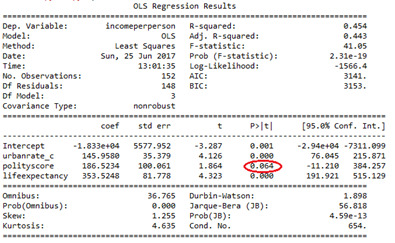
Urbanrate Squared (urbanrate_c**2)
Rejected because p-value increased to .048 when Employment rate added.

CODE
# -*- coding: utf-8 -*- """ Created June 25, 2017 @author: kbolam """ import numpy import pandas import matplotlib.pyplot as plt import statsmodels.api as sm import statsmodels.formula.api as smf import seaborn
# bug fix for display formats to avoid run time errors pandas.set_option('display.float_format', lambda x:'%.2f'%x)
data = pandas.read_csv('gapminderorig.csv')
# convert to numeric format data['incomeperperson'] = pandas.to_numeric(data['incomeperperson'], errors='coerce') data['urbanrate'] = pandas.to_numeric(data['urbanrate'], errors='coerce') data['employrate'] = pandas.to_numeric(data['employrate'], errors='coerce') data['lifeexpectancy'] = pandas.to_numeric(data['lifeexpectancy'], errors='coerce')
# listwise deletion of missing values sub1 = data[['urbanrate', 'incomeperperson', 'employrate', 'lifeexpectancy']].dropna()
# center quantitative IVs for regression analysis sub1['urbanrate_c'] = (sub1['urbanrate'] - sub1['urbanrate'].mean()) sub1['employrate_c'] = (sub1['employrate'] - sub1['employrate'].mean()) sub1['lifeexpectancy_c'] = (sub1['lifeexpectancy'] - sub1['lifeexpectancy'].mean()) sub1[["urbanrate_c", "employrate_c", "lifeexpectancy_c"]].describe()
#Best fit model # adding life expetancy, employrate reg3 = smf.ols('incomeperperson ~ urbanrate_c + lifeexpectancy_c + employrate_c', data=sub1).fit() print (reg3.summary())
#Q-Q plot for normality fig4=sm.qqplot(reg3.resid, line='r')
# simple plot of residuals stdres=pandas.DataFrame(reg3.resid_pearson) plt.plot(stdres, 'o', ls='None') l = plt.axhline(y=0, color='r') plt.ylabel('Standardized Residual') plt.xlabel('Observation Number')
# additional regression diagnostic plots # NEEDED TO ADD "=" AFTER FIGSIZE IN LINE BELOW fig2 = plt.figure(figsize=(12,8)) fig2 = sm.graphics.plot_regress_exog(reg3, "employrate_c", fig=fig2)
# additional regression diagnostic plots # NEEDED TO ADD "=" AFTER FIGSIZE IN LINE BELOW fig2 = plt.figure(figsize=(12,8)) fig2 = sm.graphics.plot_regress_exog(reg3, "lifeexpectancy_c", fig=fig2)
# additional regression diagnostic plots # NEEDED TO ADD "=" AFTER FIGSIZE IN LINE BELOW fig2 = plt.figure(figsize=(12,8)) fig2 = sm.graphics.plot_regress_exog(reg3, "urbanrate_c", fig=fig2)
# leverage plot fig3=sm.graphics.influence_plot(reg3, size=8) print(fig3)
0 notes
Text
Basics of Linear Regression
Regression Modeling in Practice, Assignment 2
1) Code
# -*- coding: utf-8 -*- """ Created on 5/21/17
@author: kbolam """
import numpy as numpy import pandas as pandas import seaborn import statsmodels.api import statsmodels.formula.api as smf import scipy import matplotlib.pyplot as plt
# Needed to change to 'latin-1" encoding so csv would load data2 = pandas.read_csv('WB_Aid_Income_growth_2015new2.csv', encoding='latin-1', low_memory=False)
#setting variables you will be working with to numeric data2['income2015'] = data2['income2015'].convert_objects(convert_numeric=True) data2['aid2015'] = data2['aid2015'].convert_objects(convert_numeric=True) #data['Urban_pop_growth'] = data['Urban_pop_growth'].convert_objects(convert_numeric=True)
#remove blank values data2['income2015']=data2['income2015'].replace(' ', numpy.nan) data2['aid2015']=data2['aid2015'].replace(' ', numpy.nan)
data2=data2.dropna()
#group income2015 into 2 catgorical variables def incomegrp (row): if row['income2015'] <= 3200: return 0 elif row['income2015'] > 3200: return 1
data2['incomegrp'] = data2.apply (lambda row: incomegrp (row),axis=1)
#print frequency table for incomegrp variable print ('Income Group: 1 = HIGH INCOME; 0 = LOW INCOME') chk1 = data2['incomegrp'].value_counts(sort=False, dropna=False) print(chk1)
#run OLS regression with fit statistics and print summary print ("OLS regression model for the association between Aid Received and Income Group") reg1 = smf.ols('aid2015 ~ incomegrp', data=data2).fit() print (reg1.summary())
2) Output
The quantitative income per capita variable (income2015) was recoded as a binary Categorical Explanatory variable (incomegrp) :
Frequency table for Income Group: 0 = LOW INCOME, 1 = HIGH INCOME:
0 65
1 66

3) Summary
F-Statistic = 1.243
P-Value = 0.267
Coefficient/beta for 'incomegrp' = 98.0134
Intercept = 108.5436
The F-Statistic is close to 1.0, which is a indicator that the null hypothesis is true, and the P-Value is over .05 which is also an indicator that the null hypothesis is true.
The linear regression model results indicate that aid received per capita is not significantly associated with the per capita income of a county.
0 notes
Text
Writing About Your Data
Regression Modeling in Practice, Assignment 1
Sample
The sample is from data available on the World Bank website. The World Bank was established in 1944 and is a partnership that works to reduce poverty and support development worldwide. The World Bank Group is headquartered in Washington, D.C., and provides countries around the world with loans and grants to support education, health, financial, agricultural and other private and public sector development. The sample includes data gathered from 218 countries.
http://www.worldbank.org/
Procedure
The World Bank collects data reported by official sources of member countries around the world to track information relating to development. Information also comes from the Organisation for Economic Co-operation and Development (OECD) National Accounts data files; the Official Development Assistance disbursement information; the United Nations World Urbanization Prospects data; and other data sources that were not provided. [Ideally I’d like to find out more information about the sources of the World Bank information and how the data is collected.]
For more information:
http://data.worldbank.org/about
Measures
Three separate World Bank data sets are used and are described below. The ODA and GDP per capita datasets are measured using “current US dollars” as opposed to “constant US dollars (see NOTE below for more information.) Current United States Dollars are used because the responses from the three datasets used to compare the relationship between Aid Received, Income and Urban Population Growth are from for one year (2015) .
Response Variable - Aid received per capita: Net Official Development Assistance (ODA) received per capita (current US $): Consists of disbursements of loans and grants by official agencies of the members of the Development Assistance Committee (DAC) and also by non-DAC countries. Not all specific data sources were provided.
Moderating Variable - Income received per capita : GDP per capita (current US $): Gross Domestic Product (GDP) per capita is is the sum of gross value added by all resident producers in the economy plus any product taxes and minus any subsidies not included in the value of the products. The data source was the World Bank national accounts data and the Organisation for Economic Co-operation and Development (OECD) data files.
Explanatory Variable: Urban population growth (annual %): Urban population refers to people living in urban areas as defined by national statistical offices. It is calculated using World Bank population estimates and urban ratios from the United Nations World Urbanization Prospects.
NOTE:
Current US Dollars: The actual value of US dollars for the year specified that is not adjusted for inflation.
Constant US Dollars: The value of US dollars adjusted to use a “constant” value for the dollar for all years included in the sample. Usually the measure used is the value of the dollar for a specific year such as 2000 or 2010. This results in a measure that is adjusted for inflation and allows for comparison of economic responses across various years.
0 notes
Text
Assignment 4 - GAPMinder
1) CODE (python)
# -*- coding: utf-8 -*- """ Created on 5/21/17
@author: kbolam """
import pandas import numpy import seaborn import scipy import matplotlib.pyplot as plt
# Needed to change to 'latin-1" encoding so csv would load data = pandas.read_csv('income_and_aid_received_WB_2010_d.csv', encoding='latin-1', low_memory=False)
#setting variables you will be working with to numeric data['Income_pp'] = data['Income_pp'].convert_objects(convert_numeric=True) data['Aid_received_pp'] = data['Aid_received_pp'].convert_objects(convert_numeric=True) data['Urban_pop_growth'] = data['Urban_pop_growth'].convert_objects(convert_numeric=True)
data['Income_pp']=data['Income_pp'].replace(' ', numpy.nan)
# Apparently can only run one scatter plot at a time. # MAYBE TRY CHANGING X AND Y -- I'M NOT SURE WHICH SHOULD BE RESPONSE AND WHICH EXPLANATORY # I THINK THAT Y IS RESPONSE AND X IS EXPLANATORY BUT CHECK NOTES IN SUMMARY FOR THIS ASSIGNMENT data_clean=data.dropna()
print ('association between Urban_pop_growth and Aid_received_pp') print (scipy.stats.pearsonr(data_clean['Urban_pop_growth'], data_clean['Aid_received_pp']))
def incomegrp (row): if row['Income_pp'] <= 660: return 1 elif row['Income_pp'] <= 2300 : return 2 elif row['Income_pp'] > 2300: return 3
data_clean['incomegrp'] = data_clean.apply (lambda row: incomegrp (row),axis=1)
chk1 = data_clean['incomegrp'].value_counts(sort=False, dropna=False) print(chk1)
sub1=data_clean[(data_clean['incomegrp']== 1)] sub2=data_clean[(data_clean['incomegrp']== 2)] sub3=data_clean[(data_clean['incomegrp']== 3)]
print ('association between urban population growth and aid received per person for LOW income countries') print (scipy.stats.pearsonr(sub1['Urban_pop_growth'], sub1['Aid_received_pp'])) print (' ') print ('association between urban population growth and aid received per person for MIDDLE income countries') print (scipy.stats.pearsonr(sub2['Urban_pop_growth'], sub2['Aid_received_pp'])) print (' ') print ('association between urban population growth and aid received per person for HIGH income countries') print (scipy.stats.pearsonr(sub3['Urban_pop_growth'], sub3['Aid_received_pp']))
''' scat1 = seaborn.regplot(x="Urban_pop_growth", y="Aid_received_pp", data=sub1) plt.xlabel('Urban Population Growth') plt.ylabel('Aid Received Per Person') plt.title('Scatterplot for the Association Between Urban Population Growth and Aid Received Per Person Rate for LOW income countries') print (scat1)
scat2 = seaborn.regplot(x="Urban_pop_growth", y="Aid_received_pp", fit_reg=False, data=sub2) plt.xlabel('Urban Population Growth') plt.ylabel('Aid Received Per Person') plt.title('Scatterplot for the Association Between Urban Population Growth and Aid Received Per Person Rate for MIDDLE income countries') print (scat2) ''' scat3 = seaborn.regplot(x="Urban_pop_growth", y="Aid_received_pp", data=sub3) plt.xlabel('Urban Population Growth') plt.ylabel('Aid Received Per Person') plt.title('Scatterplot for the Association Between Urban Population Growth and Aid Received Per Person Rate for HIGH income countries') print (scat3)
2) OUTPUT/RESULTS
For this assignment I used the Pearson R Correlation Coefficient for the inferential test using a categorical Moderating variable because both the Response and Explanatory variables are quantitative.
The quantitative variable Income Per Person was broken down into three categories to create the categorical Moderating Variable of Income Group: Low, Medium and High Income. The Pearson R Correlation Coefficient was run for each group using the following Response and Explanatory variables:
Response Variable: Aid Received Per Person (Aid_received_pp) Explanatory Variable: Urban Population Growth (Urban_pop_growth) Moderating Variable: Income Group (incomegrp) created from Income Per Person (income_pp)
R and P values WITHOUT the Moderating variable: The R value is close to -.20 and the P value is about .026 which is less than .05. The values do not indicate a very strong correlation but do indicate that there is a possible negative relationship between the two variables: R value: -0.19824330900330461 P value: 0.026065670618157444
R and P values WITH the Moderating variable:
LOW Income R value: 0.094315436858260077 P value: 0.55243551756607689) The R value at .01 is close to 0 and the P value is high at .55, so for the countries with the lowest income there is no indication of a correlation between Urban Population Growth and Aid Received Per Person.

MIDDLE Income R value: -0.21125721901189495 P value: 0.17927184082898076 The R value at -0.21 is low enough to suggest a possible negative relationship but the P value is high at .17 which indicates there is not a relationship between Urban Population Growth and Aid Received Per Person for Middle Income Countries.

HIGH Income R value: -0.28051984252791295 P value: 0.07194985469995091 The R value at -0.28 suggests a possible negative relationship but the P value is higher than 0.05 at 0.07 which indicates there is not a relationship between Urban Population Growth and Aid Received Per Person for High Income countries.
3) SUMMARY
The results of the Pearson R Correlation Coefficient tests using a Moderating Variable derived from Income Per Person indicate that there is not a relationship between Aid Received and Urban Growth, however, as I mentioned in the previous blog, the GapMinder dataset has blank values for Aid Received Per Person for the 30 countries with the highest Income Per Person. This missing data may result in misleading results. I would be interested to see if there is any significant change to the results after adding more complete Aid Received Per Person information to the dataset .
0 notes
Text
Assignment 3 - GAPMinder
1) CODE (python)
# -*- coding: utf-8 -*- """ Created on 5/21/17
@author: kbolam """
import pandas import numpy import seaborn import scipy import matplotlib.pyplot as plt
# Needed to change to 'latin-1" encoding so csv would load data = pandas.read_csv('income_and_aid_received_WB_2010.csv', encoding='latin-1', low_memory=False)
# Chose quantitative variables from GAPMINDER database # Because Pearson Correleation tool requires quantitative variables # setting quantitative variables to numeric
data['Income_pp'] = data['Income_pp'].convert_objects(convert_numeric=True)
data['Aid_received_pp'] = data['Aid_received_pp'].convert_objects(convert_numeric=True) data['Urban_pop_growth'] = data['Urban_pop_growth'].convert_objects(convert_numeric=True)
data['Income_pp']=data['Income_pp'].replace(' ', numpy.nan)
# Apparently can only run one scatter plot at a time. # Y IS RESPONSE AND X IS EXPLANATORY ''' scat1 = seaborn.regplot(x="Income_pp", y="Aid_received_pp", fit_reg=True, data=data) plt.xlabel('Income_pp') plt.ylabel('Aid_received_pp') plt.title('Scatterplot for the Association Between Income_pp and Aid_received_pp') ''' scat2 = seaborn.regplot(x="Urban_pop_growth", y="Aid_received_pp", fit_reg=True, data=data) plt.xlabel('Urban_pop_growth') plt.ylabel('Aid_received_pp') plt.title('Scatterplot for the Association Between Urban_pop_growth and Aid_received_pp')
data_clean=data.dropna()
print ('association between Income_pp and Aid_received_pp') print (scipy.stats.pearsonr(data_clean['Income_pp'], data_clean['Aid_received_pp']))
print ('association between Urban_pop_growth and Aid_received_pp') print (scipy.stats.pearsonr(data_clean['Urban_pop_growth'], data_clean['Aid_received_pp']))
2) OUTPUT and SUMMARY
Assignment 3 covers the Pearson Correlation tool for quantitative variables. For previous assignments I used the MUDF dataset that has mostly categorical variables so for this assignment I decided to use quantitative variables from the Gapminder dataset. I was interested in the following two questions and used the indicated Response and Explanatory quantitative variables to generate a correlation coefficient (R-value) using the Pearson Correlation tool:
1. Is more aid received per person in countries that have a higher income per person?
Response Variable: Aid received per person (Aid_received_pp) Explanatory Variable: Income per person (Income_pp)
R value: 0.027092283689885945 P value: 0.76331186580458943

Summary: Since the R value is close to zero and P value is greater than 0.05 the results indicate there is little or no relationship between these two variables. However, in looking at the dataset description for the “Aid received per person” variable, the aid amount included is foreign aid and does not include domestic aid received per person in more affluent countries. The 30 Countries with the highest per capita income did not report any aid received, including the U.S., Norway, Sweden, Canada and UK. Most of these 30 countries have domestic programs that provide aid to residents and this aid is not included in the Gapminder data. It would be interesting to see if the R and P values change if the data included both foreign and domestic aid received per person.
2. Does Aid received per person increase if urban population growth increases?
Response Variable: Aid received per person (Aid_received_pp) Explanatory Variable: Urban Population Growth (Urban_pop_growth)
R value: -0.19824330900330464 P value: 0.026065670618157444

Summary: Since the R value is close to -0.20 and the P value at 0.02 is less than 0.05, the results indicate there is possibly a negative relationship between the two variables: the greater the urban growth the less aid received per person. Again, as in the first test, the aid received per person variable appears to include only foreign aid, and the Aid received per person amount is blank for more affluent countries. However, given that in many less affluent areas of the world there has long been a trend of people moving from rural to urban areas, it would be interesting to explore further the possible connections between aid received and urban growth. For instance, to see if less aid is received because people’s incomes actually rise when they move to the city or if aid is more difficult for individuals to receive in urban areas because of greater bureaucracy, etc.
0 notes
Text
MUDF - Assignment 2
DATA ANALYSIS TOOLS (python)
1) CODE
# -*- coding: utf-8 -*- """ Created on 05/14/17
@author: kb """ import pandas as pd import numpy as np import scipy.stats import seaborn import matplotlib.pyplot as plt
#Had error reading csv with utf-8 encoding so changed to "ISO-8859-1" and error was resolved data = pd.read_csv('mudf_ART_df3.csv', encoding = "ISO-8859-1", low_memory=False)
#Set PANDAS to show all columns in DataFrame pd.set_option('display.max_columns', None) #Set PANDAS to show all rows in DataFrame pd.set_option('display.max_rows', None)
print ('Number of observations (rows)') print (len(data)) #number of observations (rows)
print ('Number of variables (columns)') print (len(data.columns)) # number of variables (columns)
#setting variables you will be working with to numeric AND categorical #IPEDS: Unique identifier for colleges and universities: https://nces.ed.gov/ipeds # RESPONSE VARIABLE NEEDS TO BE NUMERIC - IPEDS USED TO CREATE # EXPLANATORY VARIABLE "EDU_INST" (SEE BELOW) THAT HAS TWO VALUES # 1 = IPEDs does not equal 0, 0 = IPEDS equals 0 data['IPEDS'] = pd.to_numeric(data['IPEDS']) #LOCALE4: 1=CITY; 2=SUBURB; 03=TOWN; O4=RURAL # EXPLANATORY VARIABLE NEEDS TO BE CATEGORICAL data['LOCALE4'] = data['LOCALE4'].astype('category')
#create new column: EDU_INST=yes identifies art museums and galleriesassociated with a college or university # EDU_INST=no indicates art museums and galleries not associated with college or university #EDU_INST = yes indicates an IPEDS indentifier was included in IPEDS column (Unique identifier for colleges and universities: https://nces.ed.gov/ipeds)
data['EDU_INST'] = np.where(data['IPEDS'] > 0, 'yes', 'no')
#CREATE NUMERIC VERSION OF EDU_INST FOR CHI-SQUARED TEST AND #FOR BIVARIATE BAR CHART, EDUCATIONAL INSTITUTION "YES" = 1 data['EDU_INST_NUM'] = np.where(data['IPEDS'] > 0, 1, 0)
data['EDU_INST_NUM'] = pd.to_numeric(data['EDU_INST_NUM'], errors='coerce')
#EDU_INST_NUM was rounding to 0 and 1, so forced display of decimals to 7 places. pd.set_option('precision',7)
#recoding values for LOCALE4 into a new variable, LOCALE4_NAME recode1 = {1: "CITY", 2: "SUBURB", 3: "TOWN", 4: "RURAL"} data['LOCALE4_NAME']= data['LOCALE4'].map(recode1)
print ('Locales of Museums or Art Groups: CITY, SUBURBAN, TOWN, RURAL') ct2= data.groupby('LOCALE4_NAME').size() print (ct2) print ('Percentages for Locales') pt2 = data.groupby('LOCALE4_NAME').size() * 100 / len(data) print (pt2)
#make copy of data to use for CHI-Squared test sub6 = data.copy() #pd.options.display.float_format = '{:,.0f}'.format
# contingency table of observed counts # EDU_INST_NUM is numerical RESPONSE variable and can have only two variables, # LOCALE4_NAME is 4 level smoking frequency EXPLANATORY variable, OK to have # more than 2 values ct1=pd.crosstab(sub6['EDU_INST_NUM'], sub6['LOCALE4_NAME']) print('Counts for "0" = Art Museum, Group or Center NOT part of an Educational Institution') print('Counts for "1" = Art Museum, Group or Center IS part of an Educational Institution') print (ct1)
# column percentages # shows percent of Art Museums, Centers and Groups that are part of Educational Institutions within # each EXPLANATORY variable level colsum=ct1.sum(axis=0) colpct=ct1/colsum print('colpct values') print(colpct)
# CHI-square test for all four LOCALE4 categorical variables together print ('*') print ('CHI-Square value, P Value and Expected Counts') cs1= scipy.stats.chi2_contingency(ct1) print (cs1)
# graph percent with nicotine dependence within each smoking frequency group # BivARIATE BAR CHART WITH SMOKING FREQUENCY CATEGORIES ON X AXIS AND MEAN FOR NICOTINE DEPENDENCE # (PROPORTION OF ONES) ON THE Y AXIS seaborn.factorplot(x="LOCALE4_NAME", y="EDU_INST_NUM", data=sub6, kind="bar", ci=None, order=['TOWN','CITY','SUBURB', 'RURAL']) plt.xlabel('LOCALES of Art Museum, Group or Center') plt.ylabel('Proportion Affiliated with Educational Institution')
# 1 - BONFERRONI COMPARISON 1 OF 6 REQUIRED FOR 4 CATEGORICAL EXPLANATORY VARIABLES print ('*') print ('BONFERRONI COMPARISON - 6 Comparisons required for 4 level Categorical Explanatory Variable LOCALE4_NAME') print ('P Value Adjusted for BONFERRONI Test with 6 comparisons = .05/6 = .0833' ) print ('*') print ('BONFERRONI COMPARISON 01 of 06') recode_1 = {'TOWN': 'TOWN', 'CITY': 'CITY'} sub6['BONF_COMP01']= sub6['LOCALE4_NAME'].map(recode_1)
# contingency table of observed counts ct_1=pd.crosstab(sub6['EDU_INST_NUM'], sub6['BONF_COMP01']) print (ct_1)
# column percentages colsum1=ct_1.sum(axis=0) colpct1=ct_1/colsum1 print(colpct1)
print ('chi-square value, p value, expected counts') cs_1= scipy.stats.chi2_contingency(ct_1) print (cs_1)
# 2 - BONFERRONI COMPARISON 2 OF 6 REQUIRED FOR 4 CATEGORICAL EXPLANATORY VARIABLES print ('*') print ('BONFERRONI COMPARISON 02 of 06') recode_2 = {'TOWN': 'TOWN', 'SUBURB': 'SUBURB'} sub6['BONF_COMP02']= sub6['LOCALE4_NAME'].map(recode_2)
# contingency table of observed counts ct_2=pd.crosstab(sub6['EDU_INST_NUM'], sub6['BONF_COMP02']) print (ct_2)
# column percentages colsum2=ct_2.sum(axis=0) colpct2=ct_2/colsum2 print(colpct2)
print ('chi-square value, p value, expected counts') cs_2= scipy.stats.chi2_contingency(ct_2) print (cs_2)
# 3 - BONFERRONI COMPARISON 3 OF 6 REQUIRED FOR 4 CATEGORICAL EXPLANATORY VARIABLES print ('*') print ('BONFERRONI COMPARISON 03 of 06') recode_3 = {'TOWN': 'TOWN', 'RURAL': 'RURAL'} sub6['BONF_COMP03']= sub6['LOCALE4_NAME'].map(recode_3)
# contingency table of observed counts ct_3=pd.crosstab(sub6['EDU_INST_NUM'], sub6['BONF_COMP03']) print (ct_3)
# column percentages colsum3=ct_3.sum(axis=0) colpct3=ct_3/colsum3 print(colpct3)
print ('chi-square value, p value, expected counts') cs_3= scipy.stats.chi2_contingency(ct_3) print (cs_3)
# 4 - BONFERRONI COMPARISON 4 OF 6 REQUIRED FOR 4 CATEGORICAL EXPLANATORY VARIABLES print ('*') print ('BONFERRONI COMPARISON 04 of 06') recode_4 = {'CITY': 'CITY', 'SUBURB': 'SUBURB'} sub6['BONF_COMP04']= sub6['LOCALE4_NAME'].map(recode_4)
# contingency table of observed counts ct_4=pd.crosstab(sub6['EDU_INST_NUM'], sub6['BONF_COMP04']) print (ct_4)
# column percentages colsum4=ct_4.sum(axis=0) colpct4=ct_4/colsum4 print(colpct4)
print ('chi-square value, p value, expected counts') cs_4= scipy.stats.chi2_contingency(ct_4) print (cs_4)
# 5 - BONFERRONI COMPARISON 5 OF 6 REQUIRED FOR 4 CATEGORICAL EXPLANATORY VARIABLES print ('*') print ('BONFERRONI COMPARISON 05 of 06') recode_5 = {'CITY': 'CITY', 'RURAL': 'RURAL'} sub6['BONF_COMP05']= sub6['LOCALE4_NAME'].map(recode_5)
# contingency table of observed counts ct_5=pd.crosstab(sub6['EDU_INST_NUM'], sub6['BONF_COMP05']) print (ct_5)
# column percentages colsum5=ct_5.sum(axis=0) colpct5=ct_5/colsum5 print(colpct5)
print ('chi-square value, p value, expected counts') cs_5= scipy.stats.chi2_contingency(ct_5) print (cs_5)
# 6 - BONFERRONI COMPARISON 6 OF 6 REQUIRED FOR 4 CATEGORICAL EXPLANATORY VARIABLES print ('*') print ('BONFERRONI COMPARISON 06 of 06') recode_6 = {'SUBURB': 'SUBURB', 'RURAL': 'RURAL'} sub6['BONF_COMP06']= sub6['LOCALE4_NAME'].map(recode_6)
# contingency table of observed counts ct_6=pd.crosstab(sub6['EDU_INST_NUM'], sub6['BONF_COMP06']) print (ct_6)
# column percentages colsum6=ct_6.sum(axis=0) colpct6=ct_6/colsum6 print(colpct6)
print ('chi-square value, p value, expected counts') cs_6= scipy.stats.chi2_contingency(ct_6) print (cs_6)
pd.set_option('display.float_format', lambda x:'%f'%x)
2) Output
Number of observations (rows) 3241 Number of variables (columns) 44 Locales of Museums or Art Groups: CITY, SUBURBAN, TOWN, RURAL LOCALE4_NAME CITY 1406 RURAL 766 SUBURB 697 TOWN 372 dtype: int64 Percentages for Locales LOCALE4_NAME CITY 43.381672 RURAL 23.634681 SUBURB 21.505708 TOWN 11.477939 dtype: float64 Counts for "0" = Art Museum, Group or Center NOT part of an Educational Institution Counts for "1" = Art Museum, Group or Center IS part of an Educational Institution LOCALE4_NAME CITY RURAL SUBURB TOWN EDU_INST_NUM 0 812 173 299 236 1 594 593 398 136 colpct values LOCALE4_NAME CITY RURAL SUBURB TOWN EDU_INST_NUM 0 0.577525 0.225849 0.428981 0.634409 1 0.422475 0.774151 0.571019 0.365591 * CHI-Square value, P Value and Expected Counts (293.69549341447942, 2.302469428134087e-63, 3, array([[ 659.40141932, 359.24714594, 326.88676334, 174.4646714 ], [ 746.59858068, 406.75285406, 370.11323666, 197.5353286 ]])) * BONFERRONI COMPARISON - 6 Comparisons required for 4 categorical explanatory variables P Value for 6 comparisons = .05/6 = .0833 * BONFERRONI COMPARISON 01 of 06 BONF_COMP01 CITY TOWN EDU_INST_NUM 0 812 236 1 594 136 BONF_COMP01 CITY TOWN EDU_INST_NUM 0 0.577525 0.634409 1 0.422475 0.365591 chi-square value, p value, expected counts (3.7017091464491232, 0.054356761219197955, 1, array([[ 828.73340832, 219.26659168], [ 577.26659168, 152.73340832]])) * BONFERRONI COMPARISON 02 of 06 BONF_COMP02 SUBURB TOWN EDU_INST_NUM 0 299 236 1 398 136 BONF_COMP02 SUBURB TOWN EDU_INST_NUM 0 0.428981 0.634409 1 0.571019 0.365591 chi-square value, p value, expected counts (40.124926936766734, 2.3822961845787351e-10, 1, array([[ 348.82600561, 186.17399439], [ 348.17399439, 185.82600561]])) * BONFERRONI COMPARISON 03 of 06 BONF_COMP03 RURAL TOWN EDU_INST_NUM 0 173 236 1 593 136 BONF_COMP03 RURAL TOWN EDU_INST_NUM 0 0.225849 0.634409 1 0.774151 0.365591 chi-square value, p value, expected counts (179.77085748918901, 5.4381551717950623e-41, 1, array([[ 275.30228471, 133.69771529], [ 490.69771529, 238.30228471]])) * BONFERRONI COMPARISON 04 of 06 BONF_COMP04 CITY SUBURB EDU_INST_NUM 0 812 299 1 594 398 BONF_COMP04 CITY SUBURB EDU_INST_NUM 0 0.577525 0.428981 1 0.422475 0.571019 chi-square value, p value, expected counts (40.667018500930396, 1.8050827405875379e-10, 1, array([[ 742.77983833, 368.22016167], [ 663.22016167, 328.77983833]])) * BONFERRONI COMPARISON 05 of 06 BONF_COMP05 CITY RURAL EDU_INST_NUM 0 812 173 1 594 593 BONF_COMP05 CITY RURAL EDU_INST_NUM 0 0.577525 0.225849 1 0.422475 0.774151 chi-square value, p value, expected counts (246.02495324238402, 1.9101304289480237e-55, 1, array([[ 637.61970534, 347.38029466], [ 768.38029466, 418.61970534]])) * BONFERRONI COMPARISON 06 of 06 BONF_COMP06 RURAL SUBURB EDU_INST_NUM 0 173 299 1 593 398 BONF_COMP06 RURAL SUBURB EDU_INST_NUM 0 0.225849 0.428981 1 0.774151 0.571019 chi-square value, p value, expected counts (67.978552039659888, 1.6528364244032177e-16, 1, array([[ 247.13055366, 224.86944634], [ 518.86944634, 472.13055366]]))

3) Summary
Assignment 2 was to run a CHI-Squared Test of Independence when both the Response and Explanatory variables are categorical.
DATASET: MUDF Museum dataset of Art museums, centers and groups.
Response variable: “EDU_INST” with two values 0 = Art museum, center or group NOT affiliated with an educational institution 1 = Art museum, center of and group that IS affiliated with an educational institution
Explanatory variable: “LOCALE4” with four values TOWN, CITY , SUBURB, RURAL
Since the explanatory variable LOCALE4 has four values I used the BONFERRONI Adjustment Post Hoc test to compare all the possible unique pairs of the explanatory variable frequencies, to determine if there is a relationship between the categorical variables.
As indicated in the matrix below, the BONFERRONI Adjusted P-value = .0083, and is calculated by dividing 0.05 by six which is the number of comparisons required when there are four values for the Explanatory variable. The matrix also shows that for all but the CITY-TOWN pair comparison, the p-value for each pair is well below .0083 which indicates that there is a relationship between the pairs of categorical variables and that the null hypothesis can be rejected. This suggests that there might be a relationship between Art Museums that are affiliated with educational institutions and the type of locales where they are located.

0 notes
Text
MUDF - Assignment 1
DATA ANALYSIS TOOLS (python)
1) CODE
# -*- coding: utf-8 -*- """ Created on 05/7/17
@author: kb """ import pandas as pd import numpy as np import statsmodels.formula.api as smf import statsmodels.stats.multicomp as multi # any additional libraries would be imported here
#Had error reading csv with utf-8 encoding so changed to "ISO-8859-1" and error was resolved data = pd.read_csv('mudf_ART_df3.csv', encoding = "ISO-8859-1", low_memory=False)
#Set PANDAS to show all columns in DataFrame pd.set_option('display.max_columns', None) #Set PANDAS to show all rows in DataFrame pd.set_option('display.max_rows', None)
print ('Number of observations (rows)') print (len(data)) #number of observations (rows)
print ('Number of variables (columns)') print (len(data.columns)) # number of variables (columns)
#setting variables you will be working with to numeric #BEARAG: 1= New Englan; 2 Mid-EAST; 3=Great Lakes; 4 Plains; 5=Southeast; 6=Southwest; 7=Rocky Mountains; 8=Far West data['BEAREG'] = pd.to_numeric(data['BEAREG']) #IPEDS: Unique identifier for colleges and universities: https://nces.ed.gov/ipeds # 1 = IPEDs does not equal 0, 0 = IPEDS equals 0 data['IPEDS'] = pd.to_numeric(data['IPEDS'])
#create new column: EDU_INST=yes identifies art museums and galleriesassociated with a college or university # EDU_INST=no indicates art museums and galleries not associated with college or university #EDU_INST = yes indicates an IPEDS indentifier was included in IPEDS column (Unique identifier for colleges and universities: https://nces.ed.gov/ipeds)
data['EDU_INST'] = np.where(data['IPEDS'] > 0, 'yes', 'no')
#CREATE NUMERIC VERSION OF EDU_INST FOR BIVARIATE BAR CHART, EDUCATIONAL INSTITUTION "YES" = 1 data['EDU_INST_NUM'] = np.where(data['IPEDS'] > 0, 1, 0)
#CREATE NUMERIC VERSION OF EDU_INST FOR BIVARIATE BAR CHART, EDUCATIONAL INSTITUTION "YES" = 0 #data['EDU_INST_NUM'] = np.where(data['IPEDS'] > 0, 0, 1)
print ('Counts of Art Museums and Galleries that are associated with a college or university') pd.set_option('display.float_format', lambda x:'%f'%x) ct4= data.groupby('EDU_INST').size() print (ct4)
print ('Percentage of Art Museums and Galleries that are associated with a college or university') pt4 = data.groupby('EDU_INST').size() * 100 / len(data) print (pt4)
#recoding values for BEAREG REGIONS into a new variable, BEAREG_REGIONS
recode3 = {1: "Northeast", 2: "Eastern", 3: "Great Lakes", 4: "Plains", 5: "Southeast", 6: "Southwest", 7: "Rocky Mountains", 8: "Western"} #recode1 = {1: "CITY", 2: "SUBURB", 3: "TOWN", 4: "RURAL"} data['BEAREG_REGIONS']= data['BEAREG'].map(recode3)
print ('Counts for BEAREG Regions: 1= Northeast; 2=Eastern; 3=Great Lakes; 4 Plains; 5=Southeast; 6=Southwest; 7=Rocky Mountains; 8=Western') ct2= data.groupby('BEAREG_REGIONS').size() print (ct2) print ('Percentages for BEAREG') pt2 = data.groupby('BEAREG_REGIONS').size() * 100 / len(data) print (pt2)
#reduce to subset of values required for Frequency table to show how EDU_INST frequency in BEAREG REGIONS #use groupby to group values for EDU_INST for each of the BEAREG REGION variables sub3=data.groupby(['EDU_INST','BEAREG_REGIONS']) #print ('print edu inst name and beareg name groupby') #print (sub3)
# use size to print all four BEAREG values for each EDU_INST -- see https://community.modeanalytics.com/python/tutorial/pandas-groupby-and-python-lambda-functions/ print ('Frequency table created using Pandas size to sum number of each BEAREG Region for each EDU_INST value') sub4=sub3.size() print (sub4)
# use unstack to display BEAREG REGION values as eight columns -- see https://community.modeanalytics.com/python/tutorial/pandas-groupby-and-python-lambda-functions/ print ('Frequency table created using Pandas size, and adding unstack to reformat so BEAREG Region variables are shown as columns') sub5=sub3.size().unstack() #display nan values as 0 and float with no decimals sub5=sub5.fillna(0) pd.options.display.float_format = '{:,.0f}'.format
print (sub5) #make copies of data to use for ols tests - numeric values required for both BEAREG and EDU_INST_NUM sub6 = data.copy() #sub7 = data.copy()
# ols test using BEAREG as Quantitative Response Variable and EDU_INST_NUM as Categorial Explanatory Variable #EDU_INST_NUM: EDUCATIONAL INSTITUTION Yes=1 and No=0' #BEAREG Regions: 1= Northeast; 2=Eastern; 3=Great Lakes; 4 Plains; 5=Southeast; 6=Southwest; 7=Rocky Mountains; 8=Western model1 = smf.ols(formula='BEAREG ~ C(EDU_INST_NUM)', data=sub6) results1 = model1.fit() print (results1.summary())
# subset variables in new data frame, sub1 sub7=sub6[['EDU_INST', 'EDU_INST_NUM', 'BEAREG','GCITY', 'GSTATE']]
print ('BEAREG Regions: 1= Northeast; 2=Eastern; 3=Great Lakes; 4 Plains; 5=Southeast; 6=Southwest; 7=Rocky Mountains; 8=Western')
# print mean and st dev print ('means for BEAREG by EDUCATIONAL INSTITUTION Yes=1 and No=0') m1= sub7.groupby('BEAREG').mean() print (m1)
print ('standard deviations for BEAREG by EDU_INST: EDUCATIONAL INSTITUTION Yes=1 and No=0') sd1 = sub7.groupby('BEAREG').std() print (sd1)
# ols test using EDU_INST_NUM as Quantitative Response Variable and BEAREG as Categorial Explanatory Variable, because BEAREG has more than two values #EDU_INST_NUM: EDUCATIONAL INSTITUTION Yes=1 and No=0' #BEAREG Regions: 1= Northeast; 2=Eastern; 3=Great Lakes; 4 Plains; 5=Southeast; 6=Southwest; 7=Rocky Mountains; 8=Western
sub8= sub6[['BEAREG','EDU_INST_NUM']].dropna()
model2 = smf.ols(formula='EDU_INST_NUM ~ C(BEAREG)', data=sub8).fit() print (model2.summary()) print ('BEAREG Regions: 1= Northeast; 2=Eastern; 3=Great Lakes; 4 Plains; 5=Southeast; 6=Southwest; 7=Rocky Mountains; 8=Western')
print ('means for BEAREG Regions by EDU_INST_NUM status') m2= sub8.groupby('EDU_INST_NUM').mean() print (m2)
print ('standard deviations for BEAREG Regions by EDU_INST_NUM status') sd2 = sub8.groupby('EDU_INST_NUM').std() print (sd2)
#post hoc paired comparisons mc1 = multi.MultiComparison(sub8['EDU_INST_NUM'], sub8['BEAREG']) res1 = mc1.tukeyhsd() print(res1.summary()) #upper-case all DataFrame column names - place afer code for loading data aboave data.columns = map(str.upper, data.columns)
# bug fix for display formats to avoid run time errors - put after code for loading data above #pd.set_option('display.float_format', lambda x:'%f'%x)
2) OUTPUT
runfile('C:/Users/KMB2/Documents/Python_Wesleyan/ASS_2/C2_ASS_1_answer_03_BEAREG_final3rdcd1.py', wdir='C:/Users/KMB2/Documents/Python_Wesleyan/ASS_2')
Number of observations (rows) 3241 Number of variables (columns) 44 Counts of Art Museums and Galleries that are associated with a college or university EDU_INST no 1520 yes 1721 dtype: int64 Percentage of Art Museums and Galleries that are associated with a college or university EDU_INST no 46.899105 yes 53.100895 dtype: float64 Counts for BEAREG Regions: 1= Northeast; 2=Eastern; 3=Great Lakes; 4 Plains; 5=Southeast; 6=Southwest; 7=Rocky Mountains; 8=Western BEAREG_REGIONS Eastern 575 Great Lakes 455 Northeast 247 Plains 308 Rocky Mountains 151 Southeast 680 Southwest 300 Western 525 dtype: int64 Percentages for BEAREG BEAREG_REGIONS Eastern 17.741438 Great Lakes 14.038877 Northeast 7.621105 Plains 9.503240 Rocky Mountains 4.659056 Southeast 20.981179 Southwest 9.256402 Western 16.198704 dtype: float64 Frequency table created using Pandas size to sum number of each BEAREG Region value for each EDU_INST value EDU_INST BEAREG_REGIONS no Eastern 249 Great Lakes 208 Northeast 102 Plains 109 Rocky Mountains 81 Southeast 322 Southwest 174 Western 275 yes Eastern 326 Great Lakes 247 Northeast 145 Plains 199 Rocky Mountains 70 Southeast 358 Southwest 126 Western 250 dtype: int64 Frequency table created using Pandas size, and adding unstack to reformat so BEAREG Regions are shown as columns BEAREG_REGIONS Eastern Great Lakes Northeast Plains Rocky Mountains \ EDU_INST no 249 208 102 109 81 yes 326 247 145 199 70
BEAREG_REGIONS Southeast Southwest Western EDU_INST no 322 174 275 yes 358 126 250
TEST 1: OLS test using EDU_INST_NUM as Quantitative Response Variable with two values and BEAREG as Categorial Explanatory Variable -- BEAREG has eight values
OLS Regression Results ============================================================================== Dep. Variable: BEAREG R-squared: 0.007 Model: OLS Adj. R-squared: 0.007 Method: Least Squares F-statistic: 23.38 Date: Sun, 07 May 2017 Prob (F-statistic): 1.39e-06 Time: 16:22:02 Log-Likelihood: -7168.0 No. Observations: 3241 AIC: 1.434e+04 Df Residuals: 3239 BIC: 1.435e+04 Df Model: 1 Covariance Type: nonrobust ======================================================================================== coef std err t P>|t| [95.0% Conf. Int.] ---------------------------------------------------------------------------------------- Intercept 4.6586 0.057 82.180 0.000 4.547 4.770 C(EDU_INST_NUM)[T.1] -0.3762 0.078 -4.835 0.000 -0.529 -0.224 ============================================================================== Omnibus: 1124.999 Durbin-Watson: 0.472 Prob(Omnibus): 0.000 Jarque-Bera (JB): 174.984 Skew: 0.188 Prob(JB): 1.01e-38 Kurtosis: 1.926 Cond. No. 2.70 ==============================================================================
Warnings: [1] Standard Errors assume that the covariance matrix of the errors is correctly specified. BEAREG Regions: 1= Northeast; 2=Eastern; 3=Great Lakes; 4 Plains; 5=Southeast; 6=Southwest; 7=Rocky Mountains; 8=Western means for BEAREG by EDUCATIONAL INSTITUTION Yes=1 and No=0 EDU_INST_NUM BEAREG 1 1 2 1 3 1 4 1 5 1 6 0 7 0 8 0 standard deviations for BEAREG by EDU_INST: EDUCATIONAL INSTITUTION Yes=1 and No=0 EDU_INST_NUM BEAREG 1 0 2 0 3 0 4 0 5 0 6 0 7 1 8 0
TEST 2: OLS test using BEAREG as Quantitative Response Variable with eight value and EDU_INST_NUM as Categorial Explanatory Variable with two values
OLS Regression Results ============================================================================== Dep. Variable: EDU_INST_NUM R-squared: 0.014 Model: OLS Adj. R-squared: 0.012 Method: Least Squares F-statistic: 6.757 Date: Sun, 07 May 2017 Prob (F-statistic): 5.61e-08 Time: 16:22:02 Log-Likelihood: -2322.5 No. Observations: 3241 AIC: 4661. Df Residuals: 3233 BIC: 4710. Df Model: 7 Covariance Type: nonrobust ================================================================================== coef std err t P>|t| [95.0% Conf. Int.] ---------------------------------------------------------------------------------- Intercept 0.5870 0.032 18.600 0.000 0.525 0.649 C(BEAREG)[T.2] -0.0201 0.038 -0.532 0.595 -0.094 0.054 C(BEAREG)[T.3] -0.0442 0.039 -1.127 0.260 -0.121 0.033 C(BEAREG)[T.4] 0.0591 0.042 1.394 0.163 -0.024 0.142 C(BEAREG)[T.5] -0.0606 0.037 -1.644 0.100 -0.133 0.012 C(BEAREG)[T.6] -0.1670 0.043 -3.920 0.000 -0.251 -0.083 C(BEAREG)[T.7] -0.1235 0.051 -2.410 0.016 -0.224 -0.023 C(BEAREG)[T.8] -0.1109 0.038 -2.896 0.004 -0.186 -0.036 ============================================================================== Omnibus: 7.957 Durbin-Watson: 0.017 Prob(Omnibus): 0.019 Jarque-Bera (JB): 509.722 Skew: -0.122 Prob(JB): 2.07e-111 Kurtosis: 1.072 Cond. No. 11.4 ==============================================================================
Warnings: [1] Standard Errors assume that the covariance matrix of the errors is correctly specified. BEAREG Regions: 1= Northeast; 2=Eastern; 3=Great Lakes; 4 Plains; 5=Southeast; 6=Southwest; 7=Rocky Mountains; 8=Western means for BEAREG Regions by EDU_INST_NUM status BEAREG EDU_INST_NUM 0 5 1 4 standard deviations for BEAREG Regions by EDU_INST_NUM status BEAREG EDU_INST_NUM 0 2 1 2 Multiple Comparison of Means - Tukey HSD,FWER=0.05 ============================================= group1 group2 meandiff lower upper reject --------------------------------------------- 1 2 -0.0201 -0.1345 0.0944 False 1 3 -0.0442 -0.1631 0.0747 False 1 4 0.0591 -0.0694 0.1876 False 1 5 -0.0606 -0.1723 0.0512 False 1 6 -0.167 -0.2963 -0.0378 True 1 7 -0.1235 -0.2789 0.0319 False 1 8 -0.1109 -0.2269 0.0052 False 2 3 -0.0241 -0.1185 0.0703 False 2 4 0.0791 -0.0271 0.1854 False 2 5 -0.0405 -0.1257 0.0447 False 2 6 -0.147 -0.2541 -0.0398 True 2 7 -0.1034 -0.2409 0.0342 False 2 8 -0.0908 -0.1816 0.0 False 3 4 0.1032 -0.0078 0.2143 False 3 5 -0.0164 -0.1075 0.0747 False 3 6 -0.1229 -0.2347 -0.011 True 3 7 -0.0793 -0.2206 0.062 False 3 8 -0.0667 -0.163 0.0297 False 4 5 -0.1196 -0.223 -0.0163 True 4 6 -0.2261 -0.3481 -0.1041 True 4 7 -0.1825 -0.332 -0.0331 True 4 8 -0.1699 -0.2779 -0.0619 True 5 6 -0.1065 -0.2107 -0.0022 True 5 7 -0.0629 -0.1982 0.0724 False 5 8 -0.0503 -0.1377 0.0371 False 6 7 0.0436 -0.1065 0.1937 False 6 8 0.0562 -0.0527 0.1651 False 7 8 0.0126 -0.1263 0.1515 False ---------------------------------------------
3) SUMMARY
I don’t yet completely understand how evaluating the means and whether the means are equal affects the acceptance or rejection of the null hypothesis, so I’m not sure exactly how to interpret the test results, but I gave it a try:
BEAREG Regions: 1= Northeast; 2=Eastern; 3=Great Lakes; 4 Plains; 5=Southeast; 6=Southwest; 7=Rocky Mountains; 8=Western
EDU_INST_NUM: 1 = Art Museum, Center or Group affiliated with an educational institution 2 = Art Museum, Center or Group NOT affiliated with an educational institution
TEST 1: OLS test using EDU_INST_NUM as Quantitative Response Variable with two values and BEAREG as Categorical Explanatory Variable with eight values.

F-statistic = 23.38 I believe that this F value might be enough greater than 1.0 (which is an indicator that the null hypothesis is true) that the variation among the group means is more than you’d expect to see by chance. P-value = 1.39e-06 which is very close to 0 This p value indicates there is an almost 0 chance of observing a difference as large as observed even if the two population means are identical (the null hypothesis is true) TEST 2: OLS test using BEAREG as Quantitative Response Variable with eight values and EDU_INST_NUM as Categorical Explanatory Variable with two values. Since the Quantitative Response Variable has more than eight values I used the Tukey HSD post hoc paired comparison test.

F-statistic = 6.757
I’m not sure if this F value is greater enough than 1.0 (which is an indicator that the null hypothesis is true) that the variation among the group means is more than you’d expect to see by chance. P-value = 5.61e-08 which is very close to 0This p value indicates there is an almost 0 chance of observing a difference as large as observed even if the population means are identical (the null hypothesis is true) The Tukey test results are shown at the end of the output above and I’m still working to understand their significance and how they affect the OLS results.
0 notes
Text
MUDF - Assignment 4 (python)
1) CODE
# -*- coding: utf-8 -*- """ Created on 04/30/17
@author: kb """ import pandas as pd import numpy as np import seaborn import matplotlib.pyplot as plt # any additional libraries would be imported here
#Had error reading csv with utf-8 encoding so changed to "ISO-8859-1" and error was resolved data = pd.read_csv('mudf_ART_df3.csv', encoding = "ISO-8859-1", low_memory=False)
#Set PANDAS to show all columns in DataFrame pd.set_option('display.max_columns', None) #Set PANDAS to show all rows in DataFrame pd.set_option('display.max_rows', None)
print ('Number of observations (rows)') print (len(data)) #number of observations (rows)
print ('Number of variables (columns)') print (len(data.columns)) # number of variables (columns)
#setting variables you will be working with to numeric # update convert_objects(convert_numeric=True) which has been deprecated to pd.to_numeric(data['LOCALE4'] #lOCALE4: 1=CITY; 2=SUBURB; 03=TOWN; O4=RURAL data['LOCALE4'] = pd.to_numeric(data['LOCALE4']) #BEARAG: 1= New Englan; 2 Mid-EAST; 3=Great Lakes; 4 Plains; 5=Southeast; 6=Southwest; 7=Rocky Mountains; 8=Far West data['BEAREG'] = pd.to_numeric(data['BEAREG']) #NAICS: North American Classification system: https://www.census.gov/eos/www/naics/2017NAICS/2017_NAICS_Manual.pdf data['NAICS'] = pd.to_numeric(data['NAICS']) #IPEDS: Unique identifier for colleges and universities: https://nces.ed.gov/ipeds # 1 = IPEDs does not equal 0, 0 = IPEDS equals 0 data['IPEDS'] = pd.to_numeric(data['IPEDS'])
#ADDING TITLES print ('Counts for LOCALE4: 1=CITY; 2=SUBURB; 03=TOWN; O4=RURAL') #data['LOCALE4'] = data['LOCALE4'].astype(str) ct1= data.groupby('LOCALE4').size() print (ct1) print ('Percentages for LOCALE4') pt1 = data.groupby('LOCALE4').size() * 100 / len(data) print (pt1)
print ('Counts for BEAREG: 1= New England; 2 Mid-EAST; 3=Great Lakes; 4 Plains; 5=Southeast; 6=Southwest; 7=Rocky Mountains; 8=Far West') ct2= data.groupby('BEAREG').size() print (ct2) print ('Percentages for BEAREG') pt2 = data.groupby('BEAREG').size() * 100 / len(data) print (pt2)
data['NAICS'] = data['NAICS'].astype(str) print ('Counts for NAICS: North American Classification system for types of businesses') ct3= data.groupby('NAICS').size() print (ct3) print ('Percentages for NAICS: https://www.census.gov/eos/www/naics/2017NAICS/2017_NAICS_Manual.pdf') pt3 = data.groupby('NAICS').size() * 100 / len(data) print (pt3)
#create new column: EDU_INST=yes identifies art museums and galleriesassociated with a college or university # EDU_INST=no indicates art museums and galleries not associated with college or university #EDU_INST = yes indicates an IPEDS indentifier was included in IPEDS column (Unique identifier for colleges and universities: https://nces.ed.gov/ipeds)
data['EDU_INST'] = np.where(data['IPEDS'] > 0, 'yes', 'no')
#CREATE NUMERIC VERSION OF EDU_INST FOR BIVARIATE BAR CHART, EDUCATIONAL INSTITUTION "YES" = 1 data['EDU_INST_NUM'] = np.where(data['IPEDS'] > 0, 1, 0)
#CREATE NUMERIC VERSION OF EDU_INST FOR BIVARIATE BAR CHART, EDUCATIONAL INSTITUTION "YES" = 0 #data['EDU_INST_NUM'] = np.where(data['IPEDS'] > 0, 0, 1)
print ('Counts of Art Museums and Galleries that are associated with a college or university') pd.set_option('display.float_format', lambda x:'%f'%x) ct4= data.groupby('EDU_INST').size() print (ct4)
print ('Percentage of Art Museums and Galleries that are associated with a college or university') pt4 = data.groupby('EDU_INST').size() * 100 / len(data) print (pt4)
#recoding values for LOCALE4 into a new variable, LOCALE4_NAME recode1 = {1: "CITY", 2: "SUBURB", 3: "TOWN", 4: "RURAL"} data['LOCALE4_NAME']= data['LOCALE4'].map(recode1)
recode2 = {'519120': 'Arts Library', '611000' : 'Arts Education Center (non-accredited)', '611210': '2-Year Community College', '611310': '4-Year College or University', '611610':'4-Year Arts College (accredited)','710000':'Art Center or Association', '711100':'Performing Art Center', '712110':'Art Museum or Gallery'} data['NAICS_BASED_CATEGORY']= data['NAICS'].map(recode2)
# subset variables in new data frame, sub1 sub1=data[['MID','GZIP5', 'IPEDS', 'EDU_INST', 'NAICS', 'NAICS_BASED_CATEGORY', 'BEAREG', 'LOCALE4_NAME', 'LOCALE4', 'GCITY', 'GSTATE']]
#reduce to subset of values required for Frequency table to show how NAICS art institutions frequency in LOCALE4 areas: CITY, SUBURB, TOWN, RURAL sub2=sub1[['NAICS', 'NAICS_BASED_CATEGORY', 'LOCALE4_NAME', 'LOCALE4']]
#use groupby to group values for LOCALE4 for each of the NAICS variables sub3=sub2.groupby(['NAICS_BASED_CATEGORY','LOCALE4_NAME'])
# use size to print all four LOCALE4 values for each NAICS -- see https://community.modeanalytics.com/python/tutorial/pandas-groupby-and-python-lambda-functions/ print ('Frequency table created using Pandas size to sum number of each LOCALE4 value for each NAICS value') sub4=sub3.size() print (sub4)
# use unstack to display LOCALE4 values as four columns for each type of LOCALE4 -- see https://community.modeanalytics.com/python/tutorial/pandas-groupby-and-python-lambda-functions/ print ('Frequency table created using Pandas size, and adding unstack to reformat so LOCALE4 variables are shown as columns') sub5=sub3.size().unstack() #display nan values as 0 and float with no decimals sub5=sub5.fillna(0) pd.options.display.float_format = '{:,.0f}'.format
print (sub5) #make a copy of my new subsetted data sub6 = data.copy() sub7 = data.copy()
#univariate bar graph for categorical variables #BAR CHART PROVIDE PROPORTION OF "YES" = 1 # First change format from numeric to categorical sub6['LOCALE4_NAME'] = sub6['LOCALE4_NAME'].astype('category')
seaborn.countplot(x='LOCALE4_NAME', data=sub6) plt.xlabel('Locales of Museums or Art Groups: CITY, SUBURBAN, TOWN, RURAL') plt.title('Locales of Museums or Art Groups: CITY, SUBURBAN, TOWN, RURAL from MUDF dataset')
#Univariate histogram for quantitative variable:
#univariate bar graph for categorical variables # First change format from numeric to categorical - I THINK IT IS GOOD TO CHANGE STRING TO CATEGORIAL ALSO #BAR CHART PROVIDES PROPORTION OF WHATEVER VARIABLE IS SET TO EQUAL "1" ARE INCLUDED IN EXPLANATORY VARIABLE BINS IN THIS CASE LOCALE4 sub6['EDU_INST'] = sub6['EDU_INST'].astype('category') seaborn.countplot(x='EDU_INST', data=sub6) plt.xlabel('Educational Institution: Yes or No?') plt.title('Number of Museums and Art Groups affiliated with Educational Institutions from MUDF dataset')
# bivariate bar graph C->C WITH LABELS FOR 1 = EDUCATIONAL ART INSTITUTION seaborn.factorplot(x='LOCALE4_NAME', y='EDU_INST_NUM', data=sub6, kind="bar", ci=None) plt.xlabel('Locale of Art Museums, Centers or Group ') plt.ylabel('Educational Institution: Yes') plt.title('Locales of Museums and Art Groups Affiliated with \nEducational Institutions from MUDF dataset')
''' # bivariate bar graph C->C WITH LABELS FOR 1 = NON-EDUCATIONAL ART INSTITUTION seaborn.factorplot(x='LOCALE4_NAME', y='EDU_INST_NUM', data=sub6, kind="bar", ci=None) plt.xlabel('Locale of Art Museums, Centers or Group') plt.ylabel('Educational Institution: No') plt.title('Locales of Museums and Art Groups NOT Affiliated with \nEducational Institutions from MUDF dataset') ''' #print (sub6)
#upper-case all DataFrame column names - place afer code for loading data aboave data.columns = map(str.upper, data.columns)
# bug fix for display formats to avoid run time errors - put after code for loading data above #pd.set_option('display.float_format', lambda x:'%f'%x)
2) OUTPUT
Univariate Bar Graphs
1) Bar Graph that shows locale for all 3,241 Art Museums and Art Groups. Includes art entities that are affiliated with an educational institution and those that are not.

2) Bar Graph that shows number of Museums and Art Groups that are and are not affiliated with and educational institution.

Bivariate Bar Graph
1) Bar Graph that shows the percentage of Art Museums and Art Groups affiliated with an educational institution that are located in the four different locales.

2) Bar Graph that shows the percentage of Art Museums and Art Groups NOT affiliated with an educational institution that are located in the four different locales.

3) Description
I chose to create graphs to illustrate the relationship between the following two variables:
“EDU_INST”: The response variable that indicates which Art Museums, Centers or Groups are affiliated with educational institutions. It has two values:
Yes = Affiliated with an educational institution No = Not affiliated with an educational institution
“LOCALE4_NAME”: The explanatory variable that has four values:
CITY TOWN SUBURB RURAL
I created two views of the Bivariate Bar Graph so that I could better visualize the percentages of art entities that were affiliated with educational institutions (Graph 1) and those that are NOT affiliated with educational institutions (Graph 2). It is surprising to me that:
1) There are more art entities in RURAL locales than in SUBURB or TOWN locales.
2) Almost 80 percent of art entities in RURAL locales are affiliated with educational institutions.
As I wrote in the last blog entry, for Assignment 3, I’d like to investigate further to see in what regions of the country the art entities are located. The MUDF dataset includes a variable (”BEAREG”) that bins the U.S. into 8 different regions that should be able help me to do this.
0 notes
Text
MUDF - Assignment 3 (python)
1) CODE
# -*- coding: utf-8 -*- """ Created on 04/23/17
@author: kb """ import pandas as pd import numpy as np # any additional libraries would be imported here
#Had error reading csv with utf-8 encoding so changed to "ISO-8859-1" and error was resolved data = pd.read_csv('mudf_ART_df3.csv', encoding = "ISO-8859-1", low_memory=False)
print ('Number of observations (rows)') print (len(data)) #number of observations (rows)
print ('Number of variables (columns)') print (len(data.columns)) # number of variables (columns)
#setting variables you will be working with to numeric # update convert_objects(convert_numeric=True) which has been deprecated to pd.to_numeric(data['LOCALE4'] #lOCALE4: 1=CITY; 2=SUBURB; 03=TOWN; O4=RURAL data['LOCALE4'] = pd.to_numeric(data['LOCALE4']) #BEARAG: 1= New Englan; 2 Mid-EAST; 3=Great Lakes; 4 Plains; 5=Southeast; 6=Southwest; 7=Rocky Mountains; 8=Far West data['BEAREG'] = pd.to_numeric(data['BEAREG']) #NAICS: North American Classification system: https://www.census.gov/eos/www/naics/2017NAICS/2017_NAICS_Manual.pdf data['NAICS'] = pd.to_numeric(data['NAICS']) #IPEDS: Unique identifier for colleges and universities: https://nces.ed.gov/ipeds # 1 = IPEDs does not equal 0, 0 = IPEDS equals 0 data['IPEDS'] = pd.to_numeric(data['IPEDS'])
#ADDING TITLES print ('Counts for LOCALE4: 1=CITY; 2=SUBURB; 03=TOWN; O4=RURAL') #data['LOCALE4'] = data['LOCALE4'].astype(str) ct1= data.groupby('LOCALE4').size() print (ct1) print ('Percentages for LOCALE4') pt1 = data.groupby('LOCALE4').size() * 100 / len(data) print (pt1)
print ('Counts for BEAREG: 1= New England; 2 Mid-EAST; 3=Great Lakes; 4 Plains; 5=Southeast; 6=Southwest; 7=Rocky Mountains; 8=Far West') ct2= data.groupby('BEAREG').size() print (ct2) print ('Percentages for BEAREG') pt2 = data.groupby('BEAREG').size() * 100 / len(data) print (pt2)
data['NAICS'] = data['NAICS'].astype(str) print ('Counts for NAICS: North American Classification system for types of businesses') ct3= data.groupby('NAICS').size() print (ct3) print ('Percentages for NAICS: https://www.census.gov/eos/www/naics/2017NAICS/2017_NAICS_Manual.pdf') pt3 = data.groupby('NAICS').size() * 100 / len(data) print (pt3)
#create new column: EDU_INST=yes identifies art museums and galleriesassociated with a college or university # EDU_INST=no indicates art museums and galleries not associated with college or university #EDU_INST = yes indicates an IPEDS indentifier was included in IPEDS column (Unique identifier for colleges and universities: https://nces.ed.gov/ipeds)
data['EDU_INST'] = np.where(data['IPEDS'] > 0, 'yes', 'no')
print ('Counts of Art Museums and Galleries that are associated with a college or university')
pd.set_option('display.float_format', lambda x:'%f'%x)
ct4= data.groupby('EDU_INST').size()
print (ct4)
print ('Percentage of Art Museums and Galleries that are associated with a college or university') pt4 = data.groupby('EDU_INST').size() * 100 / len(data) print (pt4)
#recoding values for LOCALE4 into a new variable, LOCALE4_NAME recode1 = {1: "CITY", 2: "SUBURB", 3: "TOWN", 4: "RURAL"} data['LOCALE4_NAME']= data['LOCALE4'].map(recode1)
recode2 = {'519120': 'Arts Library', '611000' : 'Arts Education Center (non-accredited)', '611210': '2-Year Community College', '611310': '4-Year College or University', '611610':'4-Year Arts College (accredited)','710000':'Art Center or Association', '711100':'Performing Art Center', '712110':'Art Museum or Gallery'} data['NAICS_BASED_CATEGORY']= data['NAICS'].map(recode2)
# subset variables in new data frame, sub1 sub1=data[['MID','GZIP5', 'IPEDS', 'EDU_INST', 'NAICS', 'NAICS_BASED_CATEGORY', 'BEAREG', 'LOCALE4_NAME', 'LOCALE4', 'GCITY', 'GSTATE']]
#reduce to subset of values required for Frequency table to show how NAICS art institutions frequency in LOCALE4 areas: CITY, SUBURB, TOWN, RURAL sub2=sub1[['NAICS', 'NAICS_BASED_CATEGORY', 'LOCALE4_NAME', 'LOCALE4']]
#use groupby to group values for LOCALE4 for each of the NAICS variables sub3=sub2.groupby(['NAICS_BASED_CATEGORY','LOCALE4_NAME'])
# use size to print all four LOCALE4 values for each NAICS -- see https://community.modeanalytics.com/python/tutorial/pandas-groupby-and-python-lambda-functions/ print ('Frequency table created using Pandas size to sum number of each LOCALE4 value for each NAICS value') sub4=sub3.size() print (sub4)
# use unstack to display LOCALE4 values as four columns for each type of LOCALE4 -- see https://community.modeanalytics.com/python/tutorial/pandas-groupby-and-python-lambda-functions/ print ('Frequency table created using Pandas size, and adding unstack to reformat so LOCALE4 variables are shown as columns') sub5=sub3.size().unstack() #display nan values as 0 and float with no decimals sub5=sub5.fillna(0) pd.options.display.float_format = '{:,.0f}'.format
print (sub5)
#upper-case all DataFrame column names - place afer code for loading data aboave data.columns = map(str.upper, data.columns)
# bug fix for display formats to avoid run time errors - put after code for loading data above #pd.set_option('display.float_format', lambda x:'%f'%x)
2) OUTPUT
runfile('C:/Users/KMB2/Documents/Python_Wesleyan/ASS_2/ASS_3_codebook_03c_final_02.py', wdir='C:/Users/KMB2/Documents/Python_Wesleyan/ASS_2') Number of observations (rows) 3241 Number of variables (columns) 44 Counts for LOCALE4: 1=CITY; 2=SUBURB; 03=TOWN; O4=RURAL LOCALE4 1 1406 2 697 3 372 4 766 dtype: int64 Percentages for LOCALE4 LOCALE4 1 43 2 22 3 11 4 24 dtype: float64 Counts for BEAREG: 1= New England; 2 Mid-EAST; 3=Great Lakes; 4 Plains; 5=Southeast; 6=Southwest; 7=Rocky Mountains; 8=Far West BEAREG 1 247 2 575 3 455 4 308 5 680 6 300 7 151 8 525 dtype: int64 Percentages for BEAREG BEAREG 1 8 2 18 3 14 4 10 5 21 6 9 7 5 8 16 dtype: float64 Counts for NAICS: North American Classification system for types of businesses NAICS 519120 8 611000 7 611210 347 611310 1312 611610 101 710000 410 711000 13 711100 21 712110 1022 dtype: int64 Percentages for NAICS: https://www.census.gov/eos/www/naics/2017NAICS/2017_NAICS_Manual.pdf NAICS 519120 0 611000 0 611210 11 611310 40 611610 3 710000 13 711000 0 711100 1 712110 32 dtype: float64 Counts of Art Museums and Galleries that are associated with a college or university EDU_INST no 1520 yes 1721 dtype: int64 Percentage of Art Museums and Galleries that are associated with a college or university EDU_INST no 46.899105 yes 53.100895 dtype: float64 Frequency table created using Pandas size to sum number of each LOCALE4 value for each NAICS value NAICS_BASED_CATEGORY LOCALE4_NAME 2-Year Community College CITY 86 RURAL 152 SUBURB 94 TOWN 15 4-Year Arts College (accredited) CITY 53 RURAL 19 SUBURB 22 TOWN 7 4-Year College or University CITY 474 RURAL 425 SUBURB 292 TOWN 121 Art Center or Association CITY 187 RURAL 53 SUBURB 91 TOWN 79 Art Museum or Gallery CITY 578 RURAL 111 SUBURB 189 TOWN 144 Arts Education Center (non-accredited) CITY 2 RURAL 1 SUBURB 4 Arts Library CITY 5 TOWN 3 Performing Arts Center CITY 14 RURAL 2 SUBURB 2 TOWN 3 dtype: int64 Frequency table created using Pandas size, and adding unstack to reformat so LOCALE4 variables are shown as columns LOCALE4_NAME CITY RURAL SUBURB TOWN NAICS_BASED_CATEGORY 2-Year Community College 86 152 94 15 4-Year Arts College (accredited) 53 19 22 7 4-Year College or University 474 425 292 121 Art Center or Association 187 53 91 79 Art Museum or Gallery 578 111 189 144 Arts Education Center (non-accredited) 2 1 4 0 Arts Library 5 0 0 3 Performing Arts Center 14 2 2 3
3) DESCRIPTION
IPEDS (Integrated Postsecondary Education Data System) :
1) Values added to IPEDS (where value was missing)using values from online database wh
2) New variable EDU_INST created using IPEDS and used to create frequency table
Percentage of Art Museums and Galleries that are associated with a college or university:
EDU_INST
no 46.899105 yes 53.100895
In Assignment 2, I started to fill-in the unique IPEDS number (see Assignment 2 blog) for each listing in the MUDF dataset for art galleries and museums that were affiliated with a 2 or 4-year accredited college or university where the value was blank. Using this information I created a new variable called EDU_INST that had a “yes” value for all rows that included an IPEDS number and “no” for those that did not. Then I created a frequency table that included the percentage of all art organizations and institutions that were affiliated with an accredited college and university and those that were not. For Assignment 3, I found a few more entries that were affiliated with accredited colleges or universities and I added the appropriate IPEDS number and percentage of art museums or galleries increased slightly.
NAICS (North American Industry Classification System):
1) Values added and re-binned for NAICS and used to create new frequency table using the LOCALE4 and NAICS.
2) Both NAICS and LOCALE4 value names renamed to be more meaningful.
LOCALE4_NAME: Names replaced numbers for LOCALE4 values
1: CITY 2: SUBURB 3: TOWN 4: RURAL
NAICS_BASED_CATEGORY: New names and bins for NAICS values 611210: 2-Year Community College 611310: 4-Year Arts College (accredited) 611610: 4-Year College or University 710000: Art Center or Association 712110: Art Museum or Gallery 611000: Arts Education Center (non-accredited) 519120: Arts Library 711100: Performing Art Center
Frequency table that shows the Locale of all rows in dataset grouped by their NAICS_BASED_CATEGORY:
LOCALE4_NAME CITY RURAL SUBURB TOWN NAICS_BASED_CATEGORY 2-Year Community College 86 152 94 15 4-Year Arts College (accredited) 53 19 22 7 4-Year College or University 474 425 292 121 Art Center or Association 187 53 91 79 Art Museum or Gallery 578 111 189 144 Arts Education Center (non-accredited) 2 1 4 0 Arts Library 5 0 0 3
As I added NAICS values to rows where the value was blank I noticed that the majority of the art centers and associations had no NAICS value. I don’t think there is a NAICS category that includes these types of entities. Since this was one of the main categories I’m interested in, I decided to use “710000” which is the general NAICS category for “Arts, Entertainment, and Recreation”. So, I essentially re-binned this category and a few other NAICS categories into fewer bins for the purposes of this assignment and to provide a very general impression of the information that interests me. Since the values no longer strictly follow NAICS categories, I renamed the variable as “NAICS_BASED_CATEGORY”. One of the most interesting results of this frequency table is the number of 2 and 4-year colleges and universities with art galleries and museums that are in rural areas. I think that these schools, as well as art centers in rural areas, might have more community involvement than larger museums and universities in cities -- unfortunately I’m not sure MUDF has data that will help determine that. But I’d also like to investigate in what part of the United States these rural entities are located and MUDF should be able to help with that.
0 notes
Text
MUDF - Assignment 2
1) The Program
# -*- coding: utf-8 -*- """ Created on 04/15/17
@author: kb """ import pandas as pd import numpy as np # any additional libraries would be imported here
#Had error reading csv with utf-8 encoding so changed to "ISO-8859-1" and error was resolved data = pandas.read_csv('mudf_ART_df.csv', encoding = "ISO-8859-1", low_memory=False)
print ('Number of observations (rows)') print (len(data)) #number of observations (rows)
print ('Number of variables (columns)') print (len(data.columns)) # number of variables (columns)
#setting variables you will be working with to numeric # update convert_objects(convert_numeric=True) which has been deprecated to pd.to_numeric(data['LOCALE4'] #LOCALE4: 1=CITY; 2=SUBURB; 03=TOWN; O4=RURAL data['LOCALE4'] = pd.to_numeric(data['LOCALE4']) #BEARAG: 1= New Englan; 2 Mid-EAST; 3=Great Lakes; 4 Plains; 5=Southeast; 6=Southwest; 7=Rocky Mountains; 8=Far West data['BEAREG'] = pd.to_numeric(data['BEAREG']) #NAICS: North American Classification system: https://www.census.gov/eos/www/naics/2017NAICS/2017_NAICS_Manual.pdf data['NAICS'] = pd.to_numeric(data['NAICS']) #IPEDS: Unique identifier for colleges and universities: https://nces.ed.gov/ipeds # 1 = IPEDs does not equal 0, 0 = IPEDS equals 0 data['IPEDS'] = pd.to_numeric(data['IPEDS'])
#ADDING TITLES print ('Counts for LOCALE4: 1=CITY; 2=SUBURB; 03=TOWN; O4=RURAL') #data['LOCALE4'] = data['LOCALE4'].astype(str) ct1= data.groupby('LOCALE4').size() print (ct1) print ('Percentages for LOCALE4') pt1 = data.groupby('LOCALE4').size() * 100 / len(data) print (pt1)
print ('Counts for BEAREG: 1= New England; 2 Mid-EAST; 3=Great Lakes; 4 Plains; 5=Southeast; 6=Southwest; 7=Rocky Mountains; 8=Far West') ct2= data.groupby('BEAREG').size() print (ct2) print ('Percentages for BEAREG') pt2 = data.groupby('BEAREG').size() * 100 / len(data) print (pt2)
data['NAICS'] = data['NAICS'].astype(str) print ('Counts for NAICS: North American Classification system for types of businesses') ct3= data.groupby('NAICS').size() print (ct3) print ('Percentages for NAICS: https://www.census.gov/eos/www/naics/2017NAICS/2017_NAICS_Manual.pdf') pt3 = data.groupby('NAICS').size() * 100 / len(data) print (pt3)
#create new column: EDU_INST=yes identifies art museums and galleriesassociated with a college or university # EDU_INST=no indicates art museums and galleries not associated with college or university #EDU_INST = yes indicates an IPEDS indentifier was included in IPEDS column (Unique identifier for colleges and universities: https://nces.ed.gov/ipeds)
data['EDU_INST'] = np.where(data['IPEDS'] > 0, 'yes', 'no')
print ('Counts of Art Museums and Galleries that are associated with a college or university') ct4= data.groupby('EDU_INST').size() print (ct4)
print ('Percentage of Art Museums and Galleries that are associated with a college or university') pt4 = data.groupby('EDU_INST').size() * 100 / len(data) print (pt4)
#print(data['EDU_INST'])
#upper-case all DataFrame column names - place afer code for loading data aboave data.columns = map(str.upper, data.columns)
# bug fix for display formats to avoid run time errors - put after code for loading data above pandas.set_option('display.float_format', lambda x:'%f'%x)
2) OUTPUT
runfile('C:/Users/KMB2/Documents/Python_Wesleyan/ASS_2/ASS_2_codebook_03_final03.py', wdir='C:/Users/KMB2/Documents/Python_Wesleyan/ASS_2') Number of observations (rows) 3241 Number of variables (columns) 44 Counts for LOCALE4: 1=CITY; 2=SUBURB; 03=TOWN; O4=RURAL LOCALE4 1.000000 1404 2.000000 695 3.000000 368 4.000000 766 dtype: int64 Percentages for LOCALE4 LOCALE4 1.000000 43.319963 2.000000 21.443999 3.000000 11.354520 4.000000 23.634681 dtype: float64 Counts for BEAREG: 1= New England; 2 Mid-EAST; 3=Great Lakes; 4 Plains; 5=Southeast; 6=Southwest; 7=Rocky Mountains; 8=Far West BEAREG 1 247 2 575 3 455 4 308 5 680 6 300 7 151 8 525 dtype: int64 Percentages for BEAREG BEAREG 1 7.621105 2 17.741438 3 14.038877 4 9.503240 5 20.981179 6 9.256402 7 4.659056 8 16.198704 dtype: float64 Counts for NAICS: North American Classification system for types of businesses NAICS 512110.0 2 514120.0 8 541710.0 1 541720.0 9 611000.0 6 611110.0 5 611210.0 345 611310.0 1295 611610.0 80 611710.0 1 622110.0 1 624000.0 1 624120.0 1 624190.0 1 624230.0 1 710000.0 214 711100.0 21 711110.0 2 711130.0 4 712110.0 732 712120.0 2 712190.0 1 713940.0 2 713990.0 8 721214.0 1 813110.0 7 813211.0 8 813212.0 1 813219.0 86 813312.0 1 813319.0 5 813410.0 4 813920.0 38 nan 347 dtype: int64 Percentages for NAICS: https://www.census.gov/eos/www/naics/2017NAICS/2017_NAICS_Manual.pdf NAICS 512110.0 0.061709 514120.0 0.246837 541710.0 0.030855 541720.0 0.277692 611000.0 0.185128 611110.0 0.154273 611210.0 10.644863 611310.0 39.956803 611610.0 2.468374 611710.0 0.030855 622110.0 0.030855 624000.0 0.030855 624120.0 0.030855 624190.0 0.030855 624230.0 0.030855 710000.0 6.602900 711100.0 0.647948 711110.0 0.061709 711130.0 0.123419 712110.0 22.585622 712120.0 0.061709 712190.0 0.030855 713940.0 0.061709 713990.0 0.246837 721214.0 0.030855 813110.0 0.215983 813211.0 0.246837 813212.0 0.030855 813219.0 2.653502 813312.0 0.030855 813319.0 0.154273 813410.0 0.123419 813920.0 1.172478 nan 10.706572 dtype: float64 Counts of Art Museums and Galleries that are associated with a college or university EDU_INST no 1540 yes 1701 dtype: int64 Percentage of Art Museums and Galleries that are associated with a college or university EDU_INST no 47.516199 yes 52.483801 dtype: float64
3) Summary:
Dataset: MUDF Museum Universe Data File (https://www.imls.gov/sites/default/files/mudf_documenation_2015q3.pdf)
Variables: LOCALE4, BEAREG, NAICS, EDU_INST(IPEDS)
LOCALE4 Summary: Indicates the percentage of art galleries and museums from the dataset that are in each type of locale. LOCALE4: 1=CITY; 2=SUBURB; 03=TOWN; O4=RURAL 1 43.381672 2 21.474853 3 11.508794 4 23.634681
Not so surprisingly the highest percentage of museums are located in cities, but what was a surprise, was that about 24% were in rural areas, which suggests that these may be small community art centers that may encourage more direct community involvement in creative activity than large museums that primarily show work of professional artists.
BEAREG Summary – Percentages for BEAREG (Bureau of Economic Analysis regions) indicates the percentage of art galleries and museums from the dataset are in each of the region described below. States included in each region: 1 7.621105: New England: Connecticut, Maine, Massachusetts, New Hampshire, Rhode Island, Vermont 2 17.741438: Mid-East: Delaware, District of Columbia, Maryland, New Jersey, New York, Pennsylvania 3 14.038877: Great Lakes: Illinois, Indiana, Michigan, Ohio, Wisconsin 4 9.503240: Plains: Iowa, Kansas, Minnesota, Missouri, Nebraska, North Dakota, South Dakota 5 20.981179: Southeast: Alabama, Arkansas, Florida, Georgia, Kentucky, Louisiana, Mississippi,North Carolina, South Carolina, Tennessee, Virginia, West Virginia 6 9.256402: Southwest: Arizona, New Mexico, Oklahoma, Texas 7 4.659056: Rocky Mountains: Colorado, Idaho, Montana, Utah, Wyoming 8 16.198704: Far West: Alaska, California, Hawaii, Nevada, Oregon, Washington
Not so surprising the frequency distribution for the BEAREG variable indicates that the regions that contain the large population centers -- Mid-East, Great Lakes, Southeast and Far West, contain the highest percentages of art institutions.
NAICS Summary: North American Classification system for types of businesses (https://www.census.gov/eos/www/naics/2017NAICS/2017_NAICS_Manual.pdf). See the OUTPUT above: 11% of the rows in the dataset have no value for NAICS and there are over 30 different values. However, it might be possible to reduce the number of unique values and add values to those that don't have one. I think this variable might be able to help identify which institutions are community colleges or art centers, which are often more involved in community art projects.
EDU_INST Summary: I created this variable using the IPEDS Unique identifier for colleges and universities (https://nces.ed.gov/ipeds) to determine thepercentage of the art institutions in the dataset that are associated with a college and university. It's interesting that the distribution is close to the same for both.
Percentage of Art Museums and Galleries that are associated with a college or university). no 47.732181 yes 52.267819
0 notes
Text
MUDF Dataset
The dataset I plan to work with is from the Institute of Museum and Library Services: Museum Universe Data File FY 2015 Q3
https://data.imls.gov/Museum-Universe-Data-File/Museum-Universe-Data-File-FY-2015-Q3/ku5e-zr2b?_ga=1.150442549.207833590.1491759661
The dataset includes information about all museums in the United Stated but I plan to use only the information regarding art museums. Here is a description of the the dataset from the metadata pdf:
The Museum Universe Data File (MUDF) is a data resource that provides information about known museums and museum related organizations in the United States. The MUDF is updated and maintained by the Institute of Museum and Library Services (IMLS) and is publicly released on a regular basis. This document provides technical information about the MUDF, a list of known museums and related organizations in the United States maintained by IMLS. This data file contains descriptive information about museums in the 50 states and the District of Columbia based on public records and administrative data.
In reviewing the dataset it seems like there are mainly two types of art galleries/museums, those that show mostly local or emerging artists (including students) and those that primarily show/sell art of established artists.
While even most large museums have programs for the community, especially field trips for school age children, my hypothesis is that I think that small galleries offer more opportunities for the community to experience the creative process rather than viewing art made by others. I'm interested in determining how prevalent these community galleries are around the country, and if possible how these galleries affect the community -- do they inspire people to be more creative?
Creativity is a hard thing to measure so I'm not sure if the information in this dataset alone can answer this question. Some of the following variables included in the dataset might be useful in at least identifying the smaller institutions:
1. Income and revenue of the institution: community art galleries most likely have less income and revenue 2. College or University Galleries: usually have a student gallery 3. Longitude/Latitude: Location and size of the surrounding community: galleries in small towns often are supported by the surrounding community
A related topic that might help in answering my initial question is demographic information for the areas where galleries are located, such as, population density and per capita income. I also plan to look for a dataset(s) that includes information on creative projects in a community, such as community art programs, art walks, murals, or creative startups for new technology.
Research:
In reviewing the articles and websites below it seems like there is a move towards making larger museums more relevant to the communities, but that the efforts aren’t really going far enough. Looking at travel websites it look like smaller towns with thriving art scenes are attracting visitors.
Excerpt from ABSTRACT for "Changing values in the Art Museum"
Eilean Hooper-Greenhill, Pages 9-31 | Published online: 12 Dec 2010
http://www.tandfonline.com/doi/abs/10.1080/135272500363715
In changing times older art-museum values are coming under challenge and new emphasis is being placed on museum-audience relationships.... New roles for art museum professionals, the concept of differentiated audiences, the intervention of new voices and the exposition of new narratives offer possibilities for the reconceptualisation of art museums that are rooted in late 19th-century modernist culture.
Excerpt from ABSTRACT for "The art museum ecosystem: a new alternative model" Yuha Jung Pages 321-338 | Received 16 Sep 2010, Accepted 29 Mar 2011, Published online: 26 Aug 2011
http://www.tandfonline.com/doi/abs/10.1080/09647775.2011.603927
This paper provides a theoretical perspective on an art museum as an ecosystem.... This perspective views individuals, human societies, and nature as interconnected and interdependent through communicative networks. Museums fit nicely into this paradigm in that staff members, departments, collections, mission statements, visitors, and other cultural and educational institutions are linked together, influencing and being influenced by each other....
“Journal of Hospitality Marketing & Management” Marketing Museums and Exhibitions: What Drives the Interest of Young People Alex Gofman , Howard R. Moskowitz & Tõnis Mets Pages 601-618 | Published online: 30 Jun 2011
http://www.tandfonline.com/doi/abs/10.1080/09647770600402101
http://www.fodors.com/news/photos/15-best-small-town-museums-in-the-us#!8-norman-rockwell-museum
http://www.graphicdesigndegreehub.com/20-most-creative-small-towns-in-america/
http://ptguide.com/arts-music-theatre/art-galleries
0 notes