data-analysis21

[data-analysis21]

Running a k-means Cluster Analysis

Task

This week’s assignment involves running a k-means cluster analysis. Cluster analysis is an unsupervised machine learning method that partitions the observations in a data set into a smaller set of clusters where each observation belongs to only one cluster. The goal of cluster analysis is to group, or cluster, observations into subsets based on their similarity of responses on multiple variables. Clustering variables should be primarily quantitative variables, but binary variables may also be included.

Your assignment is to run a k-means cluster analysis to identify subgroups of observations in your data set that have similar patterns of response on a set of clustering variables.

Data

This is perhaps the best known database to be found in the pattern recognition literature. Fisher's paper is a classic in the field and is referenced frequently to this day. (See Duda & Hart, for example.) The data set contains 3 classes of 50 instances each, where each class refers to a type of iris plant. One class is linearly separable from the other 2; the latter are NOT linearly separable from each other.

Predicted attribute: class of iris plant.

Attribute Information:

sepal length in cm

sepal width in cm

petal length in cm

petal width in cm

class:

Iris Setosa

Iris Versicolour

Iris Virginica

Results

A k-means cluster analysis was conducted to identify classes of iris plants based on their similarity of responses on 4 variables that represent characteristics of the each plant bud. Clustering variables included 4 quantitative variables such as: sepal length, sepal width, petal length, and petal width.

Data were randomly split into a training set that included 70% of the observations and a test set that included 30% of the observations. Then k-means cluster analyses was conducted on the training data specifying k=3 clusters (representing three classes: Iris Setosa, Iris Versicolour, Iris Virginica), using Euclidean distance.

To describe the performance of a classifier and see what types of errors our classifier is making a confusion matrix was created. The accuracy score is 0.82, which is quite good due to the small number of observation (n=150).

Code:

import numpy as np

import pandas as pd

import matplotlib.pylab as plt

from sklearn.model_selection import train_test_split

from sklearn import datasets

from sklearn.cluster import KMeans

from sklearn.metrics import accuracy_score

from sklearn.decomposition import PCA

import seaborn as sns

%matplotlib inline

rnd_state = 3927

iris = datasets.load_iris() data = pd.DataFrame(data= np.c_[iris['data'], iris['target']], columns= iris['feature_names'] + ['target'])

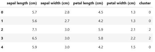
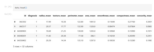
data.head()

Output:

data.info()

Output:

data.describe()

Output:

pca_transformed = PCA(n_components=2).fit_transform(data.iloc[:, :4])

colors=["#9b59b6", "#e74c3c", "#2ecc71"] plt.figure(figsize=(12,5)) plt.subplot(121) plt.scatter(list(map(lambda tup: tup[0], pca_transformed)), list(map(lambda tup: tup[1], pca_transformed)), c=list(map(lambda col: "#9b59b6" if col==0 else "#e74c3c" if col==1 else "#2ecc71", data.target))) plt.title('PCA on Iris data') plt.subplot(122) sns.countplot(data.target, palette=sns.color_palette(colors)) plt.title('Countplot Iris classes');

Output:

For visualization purposes, the number of dimensions was reduced to two by applying PCA analysis. The plot illustrates that classes 1 and 2 are not clearly divided. Countplot illustrates that our classes contain the same number of observations (n=50), so they are balanced.

(predictors_train, predictors_test, target_train, target_test) = train_test_split(data.iloc[:, :4], data.target, test_size = .3, random_state = rnd_state)

classifier = KMeans(n_clusters=3).fit(predictors_train) prediction = classifier.predict(predictors_test)

pca_transformed = PCA(n_components=2).fit_transform(predictors_test)

prediction = np.where(prediction==1, 3, prediction)

prediction = np.where(prediction==2, 1, prediction) prediction = np.where(prediction==3, 2, prediction)

plt.figure(figsize=(12,5)) plt.subplot(121) plt.scatter(list(map(lambda tup: tup[0], pca_transformed)), list(map(lambda tup: tup[1], pca_transformed)), c=list(map(lambda col: "#9b59b6" if col==0 else "#e74c3c" if col==1 else "#2ecc71", target_test))) plt.title('PCA on Iris data, real classes'); plt.subplot(122) plt.scatter(list(map(lambda tup: tup[0], pca_transformed)), list(map(lambda tup: tup[1], pca_transformed)), c=list(map(lambda col: "#9b59b6" if col==0 else "#e74c3c" if col==1 else "#2ecc71", prediction))) plt.title('PCA on Iris data, predicted classes');

Output:

clust_df = predictors_train.reset_index(level=[0]) clust_df.drop('index', axis=1, inplace=True) clust_df['cluster'] = classifier.labels_

clust_df.head()

Output:

print ('Clustering variable means by cluster') clust_df.groupby('cluster').mean()

Clustering variable means by cluster

Output:

print('Confusion matrix:\n', pd.crosstab(target_test, prediction, colnames=['Actual'], rownames=['Predicted'], margins=True)) print('\nAccuracy: ', accuracy_score(target_test, prediction))

Output:

Thanks For Reading!

[data-analysis21]

Running a Lasso Regression Analysis

Task

This week’s assignment involves running a lasso regression analysis. Lasso regression analysis is a shrinkage and variable selection method for linear regression models. The goal of lasso regression is to obtain the subset of predictors that minimizes prediction error for a quantitative response variable. The lasso does this by imposing a constraint on the model parameters that causes regression coefficients for some variables to shrink toward zero. Variables with a regression coefficient equal to zero after the shrinkage process are excluded from the model. Variables with non-zero regression coefficients variables are most strongly associated with the response variable. Explanatory variables can be either quantitative, categorical or both.

Your assignment is to run a lasso regression analysis using k-fold cross validation to identify a subset of predictors from a larger pool of predictor variables that best predicts a quantitative response variable.

Data

Dataset description: hourly rental data spanning two years.

Dataset can be found at Kaggle

Features:

yr - year

mnth - month

season - 1 = spring, 2 = summer, 3 = fall, 4 = winter

holiday - whether the day is considered a holiday

workingday - whether the day is neither a weekend nor holiday

weathersit - 1: Clear, Few clouds, Partly cloudy, Partly cloudy

2: Mist + Cloudy, Mist + Broken clouds, Mist + Few clouds, Mist

3: Light Snow, Light Rain + Thunderstorm + Scattered clouds, Light Rain + Scattered clouds

4: Heavy Rain + Ice Pallets + Thunderstorm + Mist, Snow + Fog

temp - temperature in Celsius

atemp - "feels like" temperature in Celsius

hum - relative humidity

windspeed (mph) - wind speed, miles per hour

windspeed (ms) - wind speed, metre per second

Target:

cnt - number of total rentals

Results

A lasso regression analysis was conducted to predict a number of total bikes rentals from a pool of 12 categorical and quantitative predictor variables that best predicted a quantitative response variable. Categorical predictors included weather condition and a series of 2 binary categorical variables for holiday and workingday to improve interpretability of the selected model with fewer predictors. Quantitative predictor variables include year, month, temperature, humidity and wind speed.

Data were randomly split into a training set that included 70% of the observations and a test set that included 30% of the observations. The least angle regression algorithm with k=10 fold cross validation was used to estimate the lasso regression model in the training set, and the model was validated using the test set. The change in the cross validation average (mean) squared error at each step was used to identify the best subset of predictor variables.

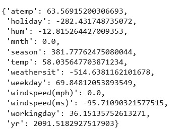
Of the 12 predictor variables, 10 were retained in the selected model:

atemp: 63.56915200306693

holiday: -282.431748735072

hum: -12.815264427009353

mnth: 0.0

season: 381.77762475080044

temp: 58.035647703871234

weathersit: -514.6381162101678

weekday: 69.84812053893549

windspeed(mph): 0.0

windspeed(ms): -95.71090321577515

workingday: 36.15135752613271

yr: 2091.5182927517903

Train data R-square 0.7899877818517489 Test data R-square 0.8131871527614188

During the estimation process, year and season were most strongly associated with the number of total bikes rentals, followed by temperature and weekday. Holiday, humidity, weather condition and wind speed (ms) were negatively associated with the number of total bikes rentals.

Code:

import pandas as pd

import numpy as np

import matplotlib.pylab as plt

from sklearn.model_selection import train_test_split

from sklearn.linear_model import LassoLarsCV

from sklearn import preprocessing

from sklearn.metrics import mean_squared_error

import seaborn as sns

%matplotlib inline

rnd_state = 983

data = pd.read_csv("data/bikes_rent.csv")

data.info()

Output:

data.describe()

Output:

data.head()

Output:

data.dropna(inplace=True)

fig, axes = plt.subplots(nrows=3, ncols=4, figsize=(20, 10)) for idx, feature in enumerate(data.columns.values[:-1]): data.plot(feature, 'cnt', subplots=True, kind='scatter', ax=axes[int(idx / 4), idx % 4], c='#87486e');

Output:

The plot above shows that there is a linear dependence between temp, atemp and cnt features. The correlations below confirm that observation.

data.iloc[:, :12].corrwith(data['cnt'])

Output:

plt.figure(figsize=(15, 5)) sns.heatmap(data[['temp', 'atemp', 'hum', 'windspeed(mph)', 'windspeed(ms)', 'cnt']].corr(), annot=True, fmt='1.4f');

Output:

There is a strong correlation between temp and atemp, as well as windspeed(mph) and windspeed(ms) features, due to the fact that they represent similar metrics in different measures. In further analysis two of those features must be dropped or applyed with penalty (L2 or Lasso regression).

predictors = data.iloc[:, :12]

target = data['cnt']

(predictors_train, predictors_test, target_train, target_test) = train_test_split(predictors, target, test_size = .3, random_state = rnd_state)

model = LassoLarsCV(cv=10, precompute=False).fit(predictors_train, target_train)

dict(zip(predictors.columns, model.coef_))

Output:

log_alphas = -np.log10(model.alphas_)

plt.figure(figsize=(10, 5))

for idx, feature in enumerate(predictors.columns): plt.plot(log_alphas, list(map(lambda r: r[idx], model.coef_path_.T)), label=feature) plt.legend(loc="upper right", bbox_to_anchor=(1.4, 0.95))

plt.xlabel("-log10(alpha)")

plt.ylabel("Feature weight")

plt.title("Lasso");

Output:

log_cv_alphas = -np.log10(model.cv_alphas_) plt.figure(figsize=(10, 5))

plt.plot(log_cv_alphas, model.mse_path_, ':')

plt.plot(log_cv_alphas, model.mse_path_.mean(axis=-1), 'k', label='Average across the folds', linewidth=2) plt.axvline(-np.log10(model.alpha_), linestyle='--', color='k', label='alpha CV') plt.legend()

plt.xlabel('-log10(alpha)')

plt.ylabel('Mean squared error')

plt.title('Mean squared error on each fold');

Output:

rsquared_train = model.score(predictors_train, target_train) rsquared_test = model.score(predictors_test, target_test)

print('Train data R-square', rsquared_train)

print('Test data R-square', rsquared_test)

Output:

Train data R-square 0.7899877818517489

Test data R-square 0.8131871527614188

Thanks For Reading!

[data-analysis21]

Running a Random Forest

Task

The second assignment deals with Random Forests. Random forests are predictive models that allow for a data driven exploration of many explanatory variables in predicting a response or target variable. Random forests provide importance scores for each explanatory variable and also allow you to evaluate any increases in correct classification with the growing of smaller and larger number of trees.

Run a Random Forest.

You will need to perform a random forest analysis to evaluate the importance of a series of explanatory variables in predicting a binary, categorical response variable.

Data

The dataset is related to red variants of the Portuguese "Vinho Verde" wine. Due to privacy and logistic issues, only physicochemical (inputs) and sensory (the output) variables are available (e.g. there is no data about grape types, wine brand, wine selling price, etc.).

The classes are ordered and not balanced (e.g. there are munch more normal wines than excellent or poor ones). Outlier detection algorithms could be used to detect the few excellent or poor wines. Also, we are not sure if all input variables are relevant. So it could be interesting to test feature selection methods.

Dataset can be found at UCI Machine Learning Repository

Attribute Information (For more information, read [Cortez et al., 2009]): Input variables (based on physicochemical tests):

1 - fixed acidity

2 - volatile acidity

3 - citric acid

4 - residual sugar

5 - chlorides

6 - free sulfur dioxide

7 - total sulfur dioxide

8 - density

9 - pH

10 - sulphates

11 - alcohol

Output variable (based on sensory data):

12 - quality (score between 0 and 10)

Results

Random forest and ExtraTrees classifier were deployed to evaluate the importance of a series of explanatory variables in predicting a categorical response variable - red wine quality (score between 0 and 10). The following explanatory variables were included: fixed acidity, volatile acidity, citric acid, residual sugar, chlorides, free sulfur dioxide, total sulfur dioxide, density, pH, sulphates and alcohol.

The explanatory variables with the highest importance score (evaluated by both classifiers) are alcohol, volatile acidity, sulphates. The accuracy of the Random forest and ExtraTrees clasifier is about 67%, which is quite good for highly unbalanced and hardly distinguished from each other classes. The subsequent growing of multiple trees rather than a single tree, adding a lot to the overall score of the model. For Random forest the number of estimators is 20, while for ExtraTrees classifier - 12, because the second classifier grows up much faster.

Code:

import pandas as pd

import numpy as np

import matplotlib.pylab as plt

from sklearn.model_selection import train_test_split, cross_val_score

from sklearn.ensemble import RandomForestClassifier, ExtraTreesClassifier

from sklearn.manifold import MDS

from sklearn.metrics.pairwise import pairwise_distances

from sklearn.metrics import accuracy_score

import seaborn as sns

%matplotlib inline

rnd_state = 4536

data = pd.read_csv('Data\wine_red.csv', sep=';')

data.info()

Output:

data.head()

Output:

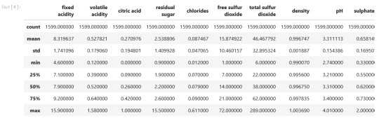
data.describe()

Output:

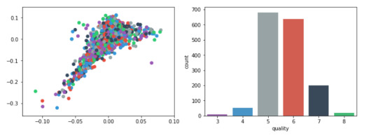
Plots

For visualization purposes, the number of dimensions was reduced to two by applying MDS method with cosine distance. The plot illustrates that our classes are not clearly divided into parts.

model = MDS(random_state=rnd_state, n_components=2, dissimilarity='precomputed')

%time representation = model.fit_transform(pairwise_distances(data.iloc[:, :11], metric='cosine'))

Wall time: 38.7 s

colors = ["#9b59b6", "#3498db", "#95a5a6", "#e74c3c", "#34495e", "#2ecc71"]

plt.figure(figsize=(12, 4))

plt.subplot(121) plt.scatter(representation[:, 0], representation[:, 1], c=colors)

plt.subplot(122) sns.countplot(x='quality', data=data, palette=sns.color_palette(colors));

Output:

predictors = data.iloc[:, :11]

target = data.quality

(predictors_train, predictors_test, target_train, target_test) = train_test_split(predictors, target, test_size = .3, random_state = rnd_state)

RandomForest classifier:

list_estimators = list(range(1, 50, 5)) rf_scoring = [] for n_estimators in list_estimators: classifier = RandomForestClassifier(random_state = rnd_state, n_jobs = -1, class_weight='balanced', n_estimators=n_estimators) score = cross_val_score(classifier, predictors_train, target_train, cv=5, n_jobs=-1, scoring = 'accuracy') rf_scoring.append(score.mean())

plt.plot(list_estimators, rf_scoring)

plt.title('Accuracy VS trees number');

Output:

classifier = RandomForestClassifier(random_state = rnd_state, n_jobs = -1, class_weight='balanced', n_estimators=20) classifier.fit(predictors_train, target_train)

Output:

RandomForestClassifier(bootstrap=True, class_weight='balanced', criterion='gini', max_depth=None, max_features='auto', max_leaf_nodes=None, min_impurity_decrease=0.0, min_impurity_split=None, min_samples_leaf=1, min_samples_split=2, min_weight_fraction_leaf=0.0, n_estimators=20, n_jobs=-1, oob_score=False, random_state=4536, verbose=0, warm_start=False)

prediction = classifier.predict(predictors_test)

print('Confusion matrix:\n', pd.crosstab(target_test, prediction, colnames=['Predicted'], rownames=['Actual'], margins=True)) print('\nAccuracy: ', accuracy_score(target_test, prediction))

feature_importance = pd.Series(classifier.feature_importances_, index=data.columns.values[:11]).sort_values(ascending=False) feature_importance

Output:

et_scoring = [] for n_estimators in list_estimators: classifier = ExtraTreesClassifier(random_state = rnd_state, n_jobs = -1, class_weight='balanced', n_estimators=n_estimators) score = cross_val_score(classifier, predictors_train, target_train, cv=5, n_jobs=-1, scoring = 'accuracy') et_scoring.append(score.mean())

plt.plot(list_estimators, et_scoring) plt.title('Accuracy VS trees number');

Output:

classifier = ExtraTreesClassifier(random_state = rnd_state, n_jobs = -1, class_weight='balanced', n_estimators=12) classifier.fit(predictors_train, target_train)

ExtraTreesClassifier(bootstrap=False, class_weight='balanced', criterion='gini', max_depth=None, max_features='auto', max_leaf_nodes=None, min_impurity_decrease=0.0, min_impurity_split=None, min_samples_leaf=1, min_samples_split=2, min_weight_fraction_leaf=0.0, n_estimators=12, n_jobs=-1, oob_score=False, random_state=4536, verbose=0, warm_start=False)

prediction = classifier.predict(predictors_test)

print('Confusion matrix:\n', pd.crosstab(target_test, prediction, colnames=['Predicted'], rownames=['Actual'], margins=True)) print('\nAccuracy: ', accuracy_score(target_test, prediction))

Output:

feature_importance = pd.Series(classifier.feature_importances_, index=data.columns.values[:11]).sort_values(ascending=False) feature_importance

Output:

Thanks For Reading!

[data-analysis21]

Running a Classification Tree

This week’s assignment involves decision trees, and more specifically, classification trees. Decision trees are predictive models that allow for a data driven exploration of nonlinear relationships and interactions among many explanatory variables in predicting a response or target variable. When the response variable is categorical (two levels), the model is a called a classification tree. Explanatory variables can be either quantitative, categorical or both. Decision trees create segmentation or subgroups in the data, by applying a series of simple rules or criteria over and over again which choose variable constellations that best predict the response (i.e. target) variable.

Run a Classification Tree.

Data

Features are computed from a digitized image of a fine needle aspirate (FNA) of a breast mass [K. P. Bennett and O. L. Mangasarian: "Robust Linear Programming Discrimination of Two Linearly Inseparable Sets", Optimization Methods and Software 1, 1992, 23-34].

In this Assignment the Decision tree has been applied to classification of breast cancer detection.

Attribute Information:

id - ID number

diagnosis (M = malignant, B = benign)

3-32 extra features

Ten real-valued features are computed for each cell nucleus: a) radius (mean of distances from center to points on the perimeter) b) texture (standard deviation of gray-scale values) c) perimeter d) area e) smoothness (local variation in radius lengths) f) compactness (perimeter^2 / area - 1.0) g) concavity (severity of concave portions of the contour) h) concave points (number of concave portions of the contour) i) symmetry j) fractal dimension ("coastline approximation" - 1)

All feature values are recorded with four significant digits. Missing attribute values: none Class distribution: 357 benign, 212 malignant

Results

Generated decision tree can be found below:

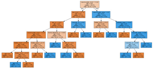
Decision tree analysis was performed to test nonlinear relationships among a series of explanatory variables and a binary, categorical response variable (breast cancer diagnosis: malignant or benign).

The dataset was splitted into train and test samples in ratio 70\30.

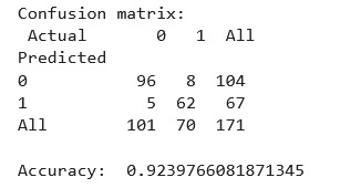
After fitting the classifier the key metrics were calculated - confusion matrix and accuracy = 0.924. This is a good result for a model trained on a small dataset.

From decision tree we can observe:

The malignant tumor is tend to have much more visible affected areas, texture and concave points, while the benign's characteristics are significantly lower.

The most important features are:

concave points_worst = 0.707688

area_worst = 0.114771

concave points_mean = 0.034234

fractal_dimension_se = 0.026301

texture_worst = 0.026300

area_se = 0.025201

concavity_se = 0.024540

texture_mean = 0.023671

perimeter_mean = 0.010415

concavity_mean = 0.006880

Code

import pandas as pd

import numpy as np

from sklearn.metrics import * from sklearn.model_selection

import train_test_split from sklearn.tree

import DecisionTreeClassifier

from sklearn import tree

from io import StringIO

from IPython.display import Image

import pydotplus

from sklearn.manifold import TSNE

from matplotlib import pyplot as plt

%matplotlib inline

rnd_state = 23467

Load data

data = pd.read_csv('Data/breast_cancer.csv')

data.info()

Output:

<class 'pandas.core.frame.DataFrame'> RangeIndex: 569 entries, 0 to 568 Data columns (total 33 columns): id 569 non-null int64 diagnosis 569 non-null object radius_mean 569 non-null float64 texture_mean 569 non-null float64 perimeter_mean 569 non-null float64 area_mean 569 non-null float64 smoothness_mean 569 non-null float64 compactness_mean 569 non-null float64 concavity_mean 569 non-null float64 concave points_mean 569 non-null float64 symmetry_mean 569 non-null float64 fractal_dimension_mean 569 non-null float64 radius_se 569 non-null float64 texture_se 569 non-null float64 perimeter_se 569 non-null float64 area_se 569 non-null float64 smoothness_se 569 non-null float64 compactness_se 569 non-null float64 concavity_se 569 non-null float64 concave points_se 569 non-null float64 symmetry_se 569 non-null float64 fractal_dimension_se 569 non-null float64 radius_worst 569 non-null float64 texture_worst 569 non-null float64 perimeter_worst 569 non-null float64 area_worst 569 non-null float64 smoothness_worst 569 non-null float64 compactness_worst 569 non-null float64 concavity_worst 569 non-null float64 concave points_worst 569 non-null float64 symmetry_worst 569 non-null float64 fractal_dimension_worst 569 non-null float64 Unnamed: 32 0 non-null float64 dtypes: float64(31), int64(1), object(1) memory usage: 146.8+ KB

In the output above there is an empty column 'Unnamed: 32', so next it should be dropped.

Plots

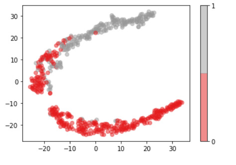
For visualization purposes, the number of dimensions was reduced to two by applying t-SNE method. The plot illustrates that our classes are not clearly divided into two parts, so the nonlinear methods (like Decision tree) may solve this problem.

model = TSNE(random_state=rnd_state, n_components=2) representation = model.fit_transform(data.iloc[:, 2:])

plt.scatter(representation[:, 0], representation[:, 1], c=data.diagnosis, alpha=0.5, cmap=plt.cm.get_cmap('Set1', 2)) plt.colorbar(ticks=range(2));

Decision tree

predictors = data.iloc[:, 2:]

target = data.diagnosis

To train a Decision tree the dataset was splitted into train and test samples in proportion 70/30.

(predictors_train, predictors_test, target_train, target_test) = train_test_split(predictors, target, test_size = .3, random_state = rnd_state)

print('predictors_train:', predictors_train.shape) print('predictors_test:', predictors_test.shape) print('target_train:', target_train.shape) print('target_test:', target_test.shape)

Output:

predictors_train: (398, 30)

predictors_test: (171, 30)

target_train: (398,)

target_test: (171,)

print(np.sum(target_train==0))

print(np.sum(target_train==1))

Output:

253

145

Our train sample is quite balanced, so there is no need in balancing it.

classifier = DecisionTreeClassifier(random_state = rnd_state).fit(predictors_train, target_train)

prediction = classifier.predict(predictors_test)

print('Confusion matrix:\n', pd.crosstab(target_test, prediction, colnames=['Actual'], rownames=['Predicted'], margins=True)) print('\nAccuracy: ', accuracy_score(target_test, prediction))

out = StringIO() tree.export_graphviz(classifier, out_file = out, feature_names = predictors_train.columns.values, proportion = True, filled = True) graph = pydotplus.graph_from_dot_data(out.getvalue()) img = Image(data = graph.create_png()) with open('output.png', 'wb') as f: f.write(img.data)

feature_importance = pd.Series(classifier.feature_importances_, index=data.columns.values[2:]).sort_values(ascending=False) feature_importance

concave points_worst 0.705688 area_worst 0.214871 concave points_mean 0.034234 fractal_dimension_se 0.028301 texture_worst 0.026300 area_se 0.025201 concavity_se 0.024540 texture_mean 0.023671 perimeter_mean 0.010415 concavity_mean 0.006880 fractal_dimension_worst 0.000000 fractal_dimension_mean 0.000000 symmetry_mean 0.000002 compactness_mean 0.005000 texture_se 0.000000 smoothness_mean 0.000000 area_mean 0.000000 radius_se 0.000000 smoothness_se 0.000000 perimeter_se 0.000001 symmetry_worst 0.000000 compactness_se 0.000000 concave points_se 0.000000 symmetry_se 0.000000 radius_worst 0.000000 perimeter_worst 0.000000 smoothness_worst 0.000000 compactness_worst 0.000002 concavity_worst 0.000000 radius_mean 0.000000 dtype: float64

#decision tree