datapheonixx-blog

[datapheonixx-blog]

Visualization of variables

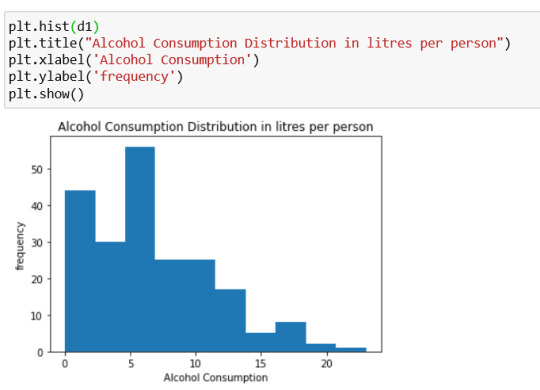
The above four histograms represent distribution of each variable.

In first histogram we observe that the maximum number of people consume alcohol in between 5 to 6.5 L (approx.). The people who are excessive drinkers are very few in number when compared to others.

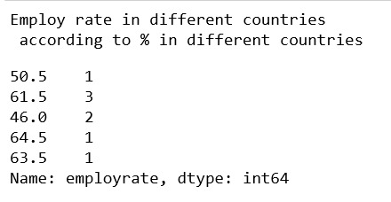
In second histogram the maximum number of females employ rate is in between 48 to 55 percent (approx.).

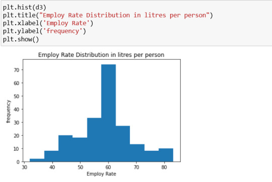
In third histogram the employ rate considering both males and females the maximum number of employ rates lie in between range of 58 and 63 percent (approx.).

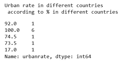
In fourth histogram we can observe that the maximum urban rate lies in between range of 58 to 62 (approx.)

Bi-variate graphs

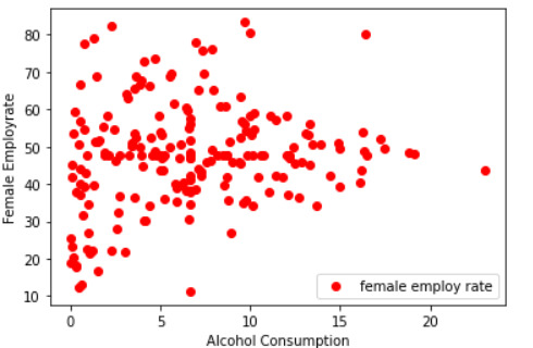
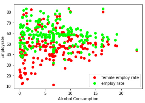
The above three scatter plots does not represent a quite significant result which is easy to interpret. But, one thing can be observed that most of the people in the dataset have an employrate between 40 to 60 percent (approx.) and out of which most of them are mediocre drinkers consuming alcohol.

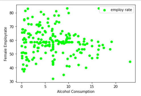
The third bi-variate graphs shows that number of the overlapping of female employ who drink alcohol and general employ rate with their alcohol consumption.

There are also outliers in gapminer data, which has been used. 

[datapheonixx-blog]

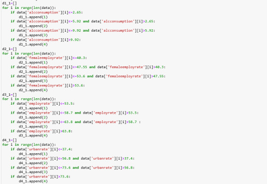
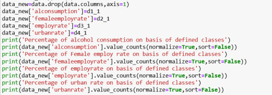
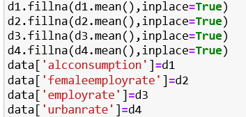
The first images shows how grouping of variables within variables have been done. The variables have been provided class labels from 1 to 4 and as class number increases from 1 to 4 the variable also tends to increase.

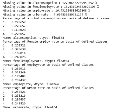
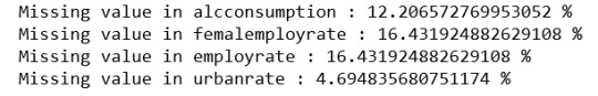
The missing data inside variables have been replaced by mean of the column as all the variables are continuous in nature.

The above frequency table highlights that all the four variables are almost equally distributed among the four classes,namely, 1,2,3,4.

[datapheonixx-blog]

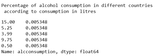
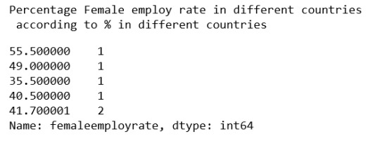
Since, the table row count of all variables were more than 100 because variable are continuous in nature, so i have shared the first five rows of each variable frequency table.

Variables

alcconsumption has a max value of 23.01, the values of classes are not equally distributed as 25 % of people drink   2.62 litres, 75% of people drink 9.92 litres, Standard Deviation = 4.89.

femaleemployrate has a max value of 83.3, the values of classes are not equally distributed as 25 % of data have employment rate 38.7, 75% of people have 55.87 , Standard Deviation = 14.62.

employrate has a max value of 83.19, the values of classes are not equally distributed as 25 % of people have employment 51.22, 75% of people have 64.97, Standard Deviation =10.51 .

urbanrate has a max value of 100, the values of classes are not equally distributed as 25 % of data lies in 36.8, 75% of data lies in 74.21, Standard Deviation =  23.84.

[datapheonixx-blog]

#Data _hidden_trends_Observation

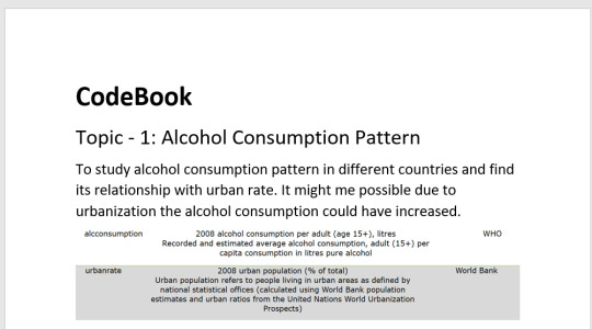
Data_set chosen for analysis and research is from gapminder.

Topic_Discovery_on: Alcohol Consumption associating with employment rate.

Variables a.k.a predictors chosen are mentioned in image one & two.

Hypothesis@ impact on alcohol intake trends due to employment .

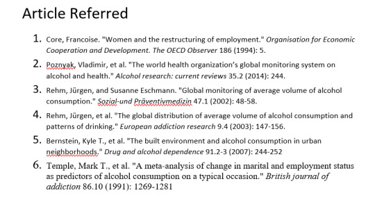
The insights i was able to draw from the topics i searched for the above mentioned variables are:- the alcohol consumption was measured as per capita consumption and average volume of consumption were divided on the basis of gender and age. Alcohol consumption worldwide is contributing to develop as one of big health concerns, as it is responsible for 3 million deaths each year and often cause disability among the age group of 15 to 49; in males, heavy drinkers account for 7.1 % global disease burden, exceeding that of female by approx 4.9%. In the paper “the built environment and alcohol consumption in urban neighborhood” conducted a survey of NYC inhabitants gathering information to understand their neighborhood of residence and studying the  alcohol consumption pattern of the city, to find a correlation.  The meta data analysis survey was done on marital and employment status with alcohol consumption, to understand the effect of heavy alcohol consumption. The marriage separation, was accompanied by heavy drinking, the major key feature which was lacking was analyzing jointly male and female drinkers, in order to derive child parenting efficiency, which has been neglected. The references are mentioned in the form of MLA citations in third image. So, my study will be focusing towards deriving relation between alcohol consumption in urban areas and change in trends of alcohol consumption due to employment rate across the globe. While i was finding research articles or work done previously on employment rate and female employ rate, many new topics arise and mostly related to fertility causing change in female employment, or employment trends suffering due to non-equality in past decades.