datasciencify-blog

[datasciencify-blog]

Logistic Regression using Python

# Logistic Regression

# Importing the libraries import numpy as np import matplotlib.pyplot as plt import pandas as pd import seaborn as sns from statsmodels.formula.api import ols import matplotlib.pyplot as plt import pylab import scipy.stats as stats import statsmodels.api as sm import statsmodels.formula.api as smf

# Importing the dataset dataset = pd.read_csv('C:/Users/Janani/Desktop/Social_Network_Ads.csv') dataset.columns = ('UserID','Gender', 'Age', 'EstimatedSalary', 'Purchased') X = dataset.iloc[:, [2, 3]].values y = dataset.iloc[:, 4].values

# Splitting the dataset into the Training set and Test set from sklearn.cross_validation import train_test_split X_train, X_test, y_train, y_test = train_test_split(X, y, test_size = 0.25, random_state = 0)

# Feature Scaling from sklearn.preprocessing import StandardScaler sc = StandardScaler() X_train = sc.fit_transform(X_train) X_test = sc.transform(X_test)

# Fitting Logistic Regression to the Training set from sklearn.linear_model import LogisticRegression classifier = LogisticRegression(random_state = 0) classifier.fit(X_train, y_train)

# Predicting the Test set results y_pred = classifier.predict(X_test)

# Making the Confusion Matrix from sklearn.metrics import confusion_matrix cm = confusion_matrix(y_test, y_pred)

# Visualising the Training set results from matplotlib.colors import ListedColormap X_set, y_set = X_train, y_train X1, X2 = np.meshgrid(np.arange(start = X_set[:, 0].min() - 1, stop = X_set[:, 0].max() + 1, step = 0.01),                     np.arange(start = X_set[:, 1].min() - 1, stop = X_set[:, 1].max() + 1, step = 0.01)) plt.contourf(X1, X2, classifier.predict(np.array([X1.ravel(), X2.ravel()]).T).reshape(X1.shape),             alpha = 0.75, cmap = ListedColormap(('red', 'green'))) plt.xlim(X1.min(), X1.max()) plt.ylim(X2.min(), X2.max()) for i, j in enumerate(np.unique(y_set)):    plt.scatter(X_set[y_set == j, 0], X_set[y_set == j, 1],                c = ListedColormap(('red', 'green'))(i), label = j) plt.title('Logistic Regression (Training set)') plt.xlabel('Age') plt.ylabel('Estimated Salary') plt.legend() plt.show()

# Visualising the Test set results from matplotlib.colors import ListedColormap X_set, y_set = X_test, y_test X1, X2 = np.meshgrid(np.arange(start = X_set[:, 0].min() - 1, stop = X_set[:, 0].max() + 1, step = 0.01),                     np.arange(start = X_set[:, 1].min() - 1, stop = X_set[:, 1].max() + 1, step = 0.01)) plt.contourf(X1, X2, classifier.predict(np.array([X1.ravel(), X2.ravel()]).T).reshape(X1.shape),             alpha = 0.75, cmap = ListedColormap(('red', 'green'))) plt.xlim(X1.min(), X1.max()) plt.ylim(X2.min(), X2.max()) for i, j in enumerate(np.unique(y_set)):    plt.scatter(X_set[y_set == j, 0], X_set[y_set == j, 1],                c = ListedColormap(('red', 'green'))(i), label = j) plt.title('Logistic Regression (Test set)') plt.xlabel('Age') plt.ylabel('Estimated Salary') plt.legend() plt.show()

model = smf.ols('Purchased ~ Gender + Age + EstimatedSalary',               data=dataset).fit() print (model.summary())

                           OLS Regression Results                             ============================================================================== Dep. Variable:              Purchased   R-squared:                       0.460 Model:                            OLS   Adj. R-squared:                  0.456 Method:                 Least Squares   F-statistic:                     112.4 Date:                Sun, 11 Nov 2018   Prob (F-statistic):           1.14e-52 Time:                        23:44:47   Log-Likelihood:                -150.16 No. Observations:                 400   AIC:                             308.3 Df Residuals:                     396   BIC:                             324.3 Df Model:                           3                                         Covariance Type:            nonrobust                                         ===================================================================================                      coef    std err          t      P>|t|      [0.025      0.975] ----------------------------------------------------------------------------------- Intercept          -0.9203      0.075    -12.268      0.000      -1.068      -0.773 Gender[T.Male]      0.0162      0.036      0.456      0.649      -0.054       0.086 Age                 0.0266      0.002     15.518      0.000       0.023       0.030 EstimatedSalary   3.84e-06   5.27e-07      7.290      0.000     2.8e-06    4.88e-06 ============================================================================== Omnibus:                       14.246   Durbin-Watson:                   1.912 Prob(Omnibus):                  0.001   Jarque-Bera (JB):                6.998 Skew:                           0.060   Prob(JB):                       0.0302 Kurtosis:                       2.363   Cond. No.                     3.33e+05 ==============================================================================

# logistic regression with Age lreg1 = smf.logit(formula = 'Purchased ~ Age', data = dataset).fit() print (lreg1.summary()) # odds ratios print ("Odds Ratios") print (np.exp(lreg1.params))

                          Logit Regression Results                           ============================================================================== Dep. Variable:              Purchased   No. Observations:                  400 Model:                          Logit   Df Residuals:                      398 Method:                           MLE   Df Model:                            1 Date:                Sun, 11 Nov 2018   Pseudo R-squ.:                  0.3553 Time:                        23:45:07   Log-Likelihood:                -168.13 converged:                       True   LL-Null:                       -260.79                                        LLR p-value:                 3.356e-42 ==============================================================================                 coef    std err          z      P>|z|      [0.025      0.975] ------------------------------------------------------------------------------ Intercept     -8.0441      0.784    -10.258      0.000      -9.581      -6.507 Age            0.1889      0.019      9.866      0.000       0.151       0.226 ============================================================================== Odds Ratios Intercept    0.000321 Age          1.207980 dtype: float64

# odd ratios with 95% confidence intervals params = lreg1.params conf = lreg1.conf_int() conf['OR'] = params conf.columns = ['Lower CI', 'Upper CI', 'OR'] print (np.exp(conf))

          Lower CI  Upper CI        OR Intercept  0.000069  0.001493  0.000321 Age        1.163476  1.254186  1.207980

# logistic regression with EstimatedSalary lreg1 = smf.logit(formula = 'Purchased ~ EstimatedSalary', data = dataset).fit() print (lreg1.summary()) # odds ratios print ("Odds Ratios") print (np.exp(lreg1.params))

                          Logit Regression Results                           ============================================================================== Dep. Variable:              Purchased   No. Observations:                  400 Model:                          Logit   Df Residuals:                      398 Method:                           MLE   Df Model:                            1 Date:                Sun, 11 Nov 2018   Pseudo R-squ.:                  0.1032 Time:                        23:45:54   Log-Likelihood:                -233.86 converged:                       True   LL-Null:                       -260.79                                        LLR p-value:                 2.168e-13 ===================================================================================                      coef    std err          z      P>|z|      [0.025      0.975] ----------------------------------------------------------------------------------- Intercept          -2.3227      0.286     -8.134      0.000      -2.882      -1.763 EstimatedSalary  2.387e-05   3.52e-06      6.790      0.000     1.7e-05    3.08e-05 =================================================================================

# odd ratios with 95% confidence intervals params = lreg1.params conf = lreg1.conf_int() conf['OR'] = params conf.columns = ['Lower CI', 'Upper CI', 'OR'] print (np.exp(conf))

                Lower CI  Upper CI        OR Intercept        0.056003  0.171521  0.098009 EstimatedSalary  1.000017  1.000031  1.000024

After adjusting for potential confounding factors (Age, Gender, Estimated Salary), the odds of having Purchased is higher. Age was also significantly associated with nicotine dependence, such that older older participants were significantly less likely to Purchase (OR=  0.000321, 95% CI=0.000069  0.001493, p=.0)

[datasciencify-blog]

Multiple Regression using Python

# Multiple Linear Regression

# Importing the libraries import numpy as np import matplotlib.pyplot as plt import pandas as pd import seaborn as sns from statsmodels.formula.api import ols import matplotlib.pyplot as plt import pylab import scipy.stats as stats import statsmodels.api as sm import statsmodels.formula.api as smf # Importing the dataset dataset = pd.read_csv('C:/Users/Janani/Desktop/50_Startups.csv') dataset.columns = ('RDSpend','Administration','MarketingSpend','State','Profit')

X = dataset.iloc[:, :-1].values y = dataset.iloc[:, 4].values # Encoding categorical data from sklearn.preprocessing import LabelEncoder, OneHotEncoder labelencoder = LabelEncoder() X[:, 3] = labelencoder.fit_transform(X[:, 3]) onehotencoder = OneHotEncoder(categorical_features = [3]) X = onehotencoder.fit_transform(X).toarray() # Avoiding the Dummy Variable Trap X = X[:, 1:] # Splitting the dataset into the Training set and Test set from sklearn.cross_validation import train_test_split X_train, X_test, y_train, y_test = train_test_split(X, y, test_size = 0.2, random_state = 0) # Fitting Multiple Linear Regression to the Training set from sklearn.linear_model import LinearRegression regressor = LinearRegression() regressor.fit(X_train, y_train) # Predicting the Test set results y_pred = regressor.predict(X_test)

stats.probplot(y_pred, dist='norm', plot=pylab) pylab.show()

model = smf.ols(formula='Profit ~ RDSpend + Administration + MarketingSpend + State' , data=dataset).fit()

model.summary()

                           OLS Regression Results                             ============================================================================== Dep. Variable:                 Profit   R-squared:                       0.951 Model:                            OLS   Adj. R-squared:                  0.945 Method:                 Least Squares   F-statistic:                     169.9 Date:                Sun, 11 Nov 2018   Prob (F-statistic):           1.34e-27 Time:                        23:00:19   Log-Likelihood:                -525.38 No. Observations:                  50   AIC:                             1063. Df Residuals:                      44   BIC:                             1074. Df Model:                           5                                         Covariance Type:            nonrobust                                         =====================================================================================                        coef    std err          t      P>|t|      [0.025      0.975] ------------------------------------------------------------------------------------- Intercept          5.013e+04   6884.820      7.281      0.000    3.62e+04     6.4e+04 State[T.Florida]    198.7888   3371.007      0.059      0.953   -6595.030    6992.607 State[T.New York]   -41.8870   3256.039     -0.013      0.990   -6604.003    6520.229 RDSpend               0.8060      0.046     17.369      0.000       0.712       0.900 Administration       -0.0270      0.052     -0.517      0.608      -0.132       0.078 MarketingSpend        0.0270      0.017      1.574      0.123      -0.008       0.062 ============================================================================== Omnibus:                       14.782   Durbin-Watson:                   1.283 Prob(Omnibus):                  0.001   Jarque-Bera (JB):               21.266 Skew:                          -0.948   Prob(JB):                     2.41e-05 Kurtosis:                       5.572   Cond. No.                     1.45e+06 ==============================================================================

model_fitted_y = model.fittedvalues plt.hist(model_fitted_y.pearson_resid) model_residuals = model.resid model_norm_residuals = model.get_influence().resid_studentized_internal model_norm_residuals_abs_sqrt = np.sqrt(np.abs(model_norm_residuals)) model_abs_resid = np.abs(model_residuals)

model_leverage = model.get_influence().hat_matrix_diag model_cooks = model.get_influence().cooks_distance[0] stats.probplot(model, dist="norm", plot=pylab) pylab.show()

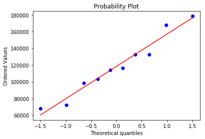
#Q-Q plot for normality fig4=sm.qqplot(model.resid, line='r')

The qq-plot clearly displays the points lie along the line and it clearly indicates there are no skewness. There are no outliers.

fig, ax = plt.subplots(figsize=(12,8)) fig = sm.graphics.influence_plot(model, ax=ax, criterion="cooks")

Influence Leverage Plot:

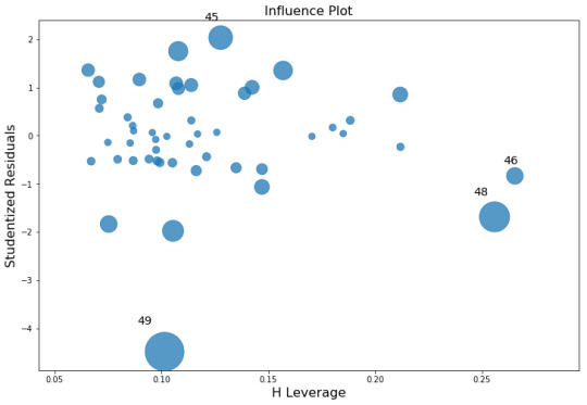
There are only three outliers hence there are not many influencers to skew the data.

# simple plot of residuals

stdres=pd.DataFrame(model.resid_pearson) plt.plot(stdres, 'o', ls='None') l = plt.axhline(y=0, color='r') plt.ylabel('Standardized Residual') plt.xlabel('Observation Number')

After adjusting for potential confounding factors R&D Spend, Administration, Marketing, State), Profit significantly increased. 

[datasciencify-blog]

Data Management and Visualization - Week 3

import numpy as np import matplotlib.pyplot as plt import pandas as pan from sklearn.cross_validation import train_test_split from sklearn.tree import DecisionTreeClassifier from sklearn.metrics import classification_report import sklearn.metrics from io import BytesIO as StringIO from sklearn import datasets import math from pylab import * import seaborn as sb #reading the first data data= pan.read_csv('Women-API-Enroll.csv')

#structure of data data.dtypes data.shape (111, 48)

#find if there are any missing data data.info()

#Find count of missing data as a whole data.isnull().sum()

#Find columns that have missing data data.columns[data.isnull().any()]

data.isnull().sum() Out[11]: Country ID           0 Region 1 - ID        0 Region 1 - Enroll    0 Region 2             0 Income Group         0 Country              0 1970                 0 1971                 0 1972                 0 1973                 0 1974                 0 1975                 0 1976                 0 1977                 0 1978                 0 1979                 0 1980                 0 1981                 0 1982                 0 1983                 0 1984                 0 1985                 0 1986                 0 1987                 0 1988                 0 1989                 0 1990                 0 1991                 0 1992                 0 1993                 1 1994                 1 1995                 0 1996                 0 1997                 1 1998                 1 1999                 0 2000                 0 2001                 2 2002                 0 2003                 1 2004                 0 2005                 0 2006                 0 2007                 0 2008                 0 2009                 0 #Find count of missing values in a column data['Income Group'].isnull().sum()

5 #fill missing data data.fillna("0")

#drop missing data data.dropna()

#select columns in data data.loc[1:5,['Income Group','Region 2']]

 Income Group               Region 2 1  High income  Europe & Central Asia 2  High income  Europe & Central Asia 3  High income          North America 4  High income  Europe & Central Asia 5  High income  Europe & Central Asia

data.loc[100:120]

   Country ID Region 1 - ID   Region 1 - Enroll  ...   2007  2008  2009 100       C101            R6  Sub-Saharan Africa  ...   34.8  34.8  39.2 101       C102            R6  Sub-Saharan Africa  ...   12.4  12.4   9.7 102       C103            R6  Sub-Saharan Africa  ...   18.0  18.0  18.0 103       C104            R6  Sub-Saharan Africa  ...   12.9  12.9  12.9 104       C105            R6  Sub-Saharan Africa  ...   32.8  32.8  43.5 105       C106            R6  Sub-Saharan Africa  ...    0.0   0.0   0.0 106       C107            R6  Sub-Saharan Africa  ...   10.8  13.8  13.8 107       C108            R6  Sub-Saharan Africa  ...    8.6   8.6   8.6 108       C109            R6  Sub-Saharan Africa  ...   29.7  29.7  29.7 109       C110            R6  Sub-Saharan Africa  ...   14.6  14.6  14.6 110       C111            R6  Sub-Saharan Africa  ...   16.7  15.2  15.2

print(“How many Regions the countries are categorized into?”) print(data['Region 1 - Enroll’].value_counts(sort = False)) Eastern Europe                                 8 Asia and the Pacific                         16 Middle East and North Africa           13 Sub-Saharan Africa                          24 Latin America and the Caribbean     26 Advanced Economies                       24

#reading the second data data_2= pan.read_csv(“Enroll - 1970 - 2010.csv”) #structure of data data_2.dtypes data_2.shape

#columns in dataset data_2.columns Index(['Country ID’, 'Country’, 'Year’, 'No Schooling’, 'Primary - Enrolled’,       'Primary - Attained’, 'Secondary - Enrolled’, 'Secondary - Attained’,       'Tertiary - Enrolled’, 'Tertiary - Attained’,       'Avg. Years of Total Schooling’, 'Avg. Years of Primary Schooling’,       'Avg. Years of Secondary Schooling’,       'Avg. Years of Tertiary\n Schooling’, 'Population\n(1000s)’, 'Region’,       'Region ID’],      dtype='object’)

print(“What are the conutries where the 'Primary - Attained’ is greater than 60%?”) a = (data_2['Country’][data_2['Primary - Attained’]>60.0 ])

print(a.unique().tolist()) What are the conutries where the 'Primary - Attained’ is greater than 20%? Country Code     Country 145              Norway 387              Hungary 450              Belize There are only three countries out of the whole set to have atleast 60% of female who attained Primary Education

[datasciencify-blog]

Linear Regression using Python

Predicting Medical Expenses 

The file dataset has 30 examples of salary and years of experience. I am trying to predict salary using years of experience.

# Importing the libraries

import numpy as np import matplotlib.pyplot as plt import pandas as pd

# Importing the dataset data = pd.read_csv('Salary_Data.csv') #structure of data data.dtypes

YearsExperience    float64 Salary             float64

data.shape

#find columns in the dataset data.columns (30, 2)

#describe data data.describe() data.info()

#check for missing data data.isnull().sum() data.columns.isnull().any()

#select numeric columns numerics = ['int16', 'int32', 'int64', 'float16', 'float32', 'float64'] numeric_data=data.select_dtypes(include=numerics)

#plot a correlation plot plt.matshow(numeric_data.corr()) plt.xticks(range(len(numeric_data.columns)),range(len(numeric_data.columns))) plt.yticks(range(len(numeric_data.columns)),numeric_data.columns) plt.colorbar() plt.show()

X = data.iloc[:, :-1].values y = data.iloc[:, 1].values

# Splitting the dataset into the Training set and Test set from sklearn.cross_validation import train_test_split X_train, X_test, y_train, y_test = train_test_split(X, y, test_size = 1/3, random_state = 0)

# Fitting Simple Linear Regression to the Training set from sklearn.linear_model import LinearRegression regressor = LinearRegression() regressor.fit(X_train, y_train)

# Predicting the Test set results y_pred = regressor.predict(X_test)

# Visualising the Training set results plt.scatter(X_train, y_train, color = 'red') plt.plot(X_train, regressor.predict(X_train), color = 'blue') plt.title('Salary vs Experience (Training set)') plt.xlabel('Years of Experience') plt.ylabel('Salary') plt.show()

# Visualising the Test set results plt.scatter(X_test, y_test, color = 'red') plt.plot(X_train, regressor.predict(X_train), color = 'blue') plt.title('Salary vs Experience (Test set)') plt.xlabel('Years of Experience') plt.ylabel('Salary') plt.show()

The salary and years of experience features are positively correlated. We can see in both training and test sets the salary increases as years of experience increases.

scat1 = sb.regplot(x="YearsExperience", y="Salary", scatter=True, data=data) plt.xlabel('Years of Experience') plt.ylabel('Salary') plt.title ('Scatterplot for the Association Between Salary and Years of Experience') print(scat1)

print ("OLS regression model for the association between Salary and Years of Experience") reg1 = smf.ols('Salary ~ YearsExperience', data=data).fit() print (reg1.summary())

OLS regression model for the association between Salary and Years of Experience                            OLS Regression Results                             ============================================================================== Dep. Variable:                 Salary   R-squared:                       0.957 Model:                            OLS   Adj. R-squared:                  0.955 Method:                 Least Squares   F-statistic:                     622.5 Date:                Mon, 05 Nov 2018   Prob (F-statistic):           1.14e-20 Time:                        21:09:14   Log-Likelihood:                -301.44 No. Observations:                  30   AIC:                             606.9 Df Residuals:                      28   BIC:                             609.7 Df Model:                           1                                         Covariance Type:            nonrobust                                         ===================================================================================                      coef    std err          t      P>|t|      [0.025      0.975] ----------------------------------------------------------------------------------- Intercept        2.579e+04   2273.053     11.347      0.000    2.11e+04    3.04e+04 YearsExperience  9449.9623    378.755     24.950   ��  0.000    8674.119    1.02e+04 ============================================================================== Omnibus:                        2.140   Durbin-Watson:                   1.648 Prob(Omnibus):                  0.343   Jarque-Bera (JB):                1.569 Skew:                           0.363   Prob(JB):                        0.456 Kurtosis:                       2.147   Cond. No.                         13.2 ==============================================================================

[datasciencify-blog]

Data Management and Visualization - Week 2

# -*- coding: utf-8 -*- """ Created on Sat Nov  3 19:38:53 2018

@author: Janani """

import numpy as np import matplotlib.pyplot as plt import pandas as pan from sklearn.cross_validation import train_test_split from sklearn.tree import DecisionTreeClassifier from sklearn.metrics import classification_report import sklearn.metrics from io import BytesIO as StringIO from sklearn import datasets import math from pylab import * import seaborn as sb

#reading the first data data= pan.read_csv("C:/Users/Janani/Desktop/Imp - DS/My Southampton/Data Visulaization/Data/Data Final/Women-API-Enroll.csv") #structure of data data.dtypes data.shape (111, 48)

#columns in dataset data.columns

['Country ID', 'Region 1 - ID', 'Region 1 - Enroll', 'Region 2',        'Income Group', 'Country', '1970', '1971', '1972', '1973', '1974',        '1975', '1976', '1977', '1978', '1979', '1980', '1981', '1982', '1983',        '1984', '1985', '1986', '1987', '1988', '1989', '1990', '1991', '1992',        '1993', '1994', '1995', '1996', '1997', '1998', '1999', '2000', '2001',        '2002', '2003', '2004', '2005', '2006', '2007', '2008', '2009', '2010',        'Unnamed: 47'],       dtype='object')

#describe data data.describe()              1970        1971     ...             2010  Unnamed: 47 count  111.000000  111.000000     ...       111.000000          0.0 mean     1.963964    3.094595     ...        18.768468          NaN std      4.928337    6.118271     ...        11.076478          NaN min      0.000000    0.000000     ...         0.000000          NaN 25%      0.000000    0.000000     ...        10.650000          NaN 50%      0.000000    0.000000     ...        16.800000          NaN 75%      1.550000    3.600000     ...        25.400000          NaN max     30.500000   30.500000     ...        45.000000          NaN data.info()

#check for missing data data.isnull().sum() data.columns.isnull().any()

data['Country'].describe() count        111 unique       111 top       Canada freq           1 Name: Country, dtype: object

print("How many Income Groups the countries are categorized into?") print(data['Income Group'].value_counts(sort = False))

Lower middle income    24 Upper middle income    32 High income                  37 Low income                   18

print("How many Regions the countries are categorized into?") print(data['Region 1 - Enroll'].value_counts(sort = False))

Eastern Europe                                 8 Asia and the Pacific                         16 Middle East and North Africa           13 Sub-Saharan Africa                          24 Latin America and the Caribbean     26 Advanced Economies                       24

#reading the first data data_2= pan.read_csv("Enroll - 1970 - 2010.csv") #structure of data data_2.dtypes data_2.shape

(999, 17)

#columns in dataset data_2.columns

Index(['Country ID', 'Country', 'Year', 'No Schooling', 'Primary - Enrolled',        'Primary - Attained', 'Secondary - Enrolled', 'Secondary - Attained',        'Tertiary - Enrolled', 'Tertiary - Attained',        'Avg. Years of Total Schooling', 'Avg. Years of Primary Schooling',        'Avg. Years of Secondary Schooling',        'Avg. Years of Tertiary\n Schooling', 'Population\n(1000s)', 'Region',        'Region ID'],       dtype='object')

print("What are the conutries where the 'Primary - Attained' is greater than 60%?") a = (data_2['Country'][data_2['Primary - Attained']>60.0 ]) print(a.unique().tolist())

What are the conutries where the 'Primary - Attained' is greater than 20%? Country Code     Country 145              Norway 387              Hungary 450              Belize

There are only three countries out of the whole set to have atleast 60% of female who attained Primary Education

print("What are the Countries where the 'Tertiary - Attained' is greater than 30%?") print(data_2['Country'][data_2['Tertiary - Attained']>30.0].unique().tolist())

What are the Countries where the 'Tertiary - Attained' is greater than 30%? Country Code Country 35                   Canada 80                   Greece 98                   Ireland 205                 USA 332                 Korea, North 341                 Korea, South There are only six countries out of the whole set to have atleast 30% of female who attained Tertiary Education between 1970 to 2010 which is very alarming.

print("What are the Regions where the 'Secondary - Attained' is greater than 40%?") a = (data_2['Region'][data_2['Secondary - Attained']>40.0 ]) print(a.unique().tolist())

What are the Regions where the 'Secondary - Attained' is greater than 40%?

Region

Advanced Economies Asia and the Pacific Eastern Europe Latin America the Caribbean Sub-Saharan Africa

If we take count Region wise then the above regions have atleast 40% of

female who attained Secondary Education between 1970 to 2010.

[datasciencify-blog]

Data Management and Visualization - Week 1

My research is to find if there exists a pattern or a relationship between women in parliament and the literacy rate of women across the globe. The dataset I have utilized for this research is “Women's Representation in National Parliaments 1970-2010” from Finnish Social Science Data Archive. “The data contain information on the percentage share of women representatives in national parliaments from the year 1970 to the year 2010. In case of a bicameral parliament, only the lower house is taken into account. The data are based on the results of parliamentary elections. After an election, the percentage share of women is taken to remain the same until the next election or as long as the parliament is operating.”[1]

Link to Dataset: http://urn.fi/urn:nbn:fi:fsd:T-FSD2183

I need to find out if the women representation in politics increased with the increase literacy rate of women across the world. The dataset consists of one column for “Country” and rest of the columns are for each year between 1970-2010. I have decided to take all the columns into consideration for analysis.

Codebook: “Women's Representation in National Parliaments 1970-2010”

Country – Lists all the countries across the globe

There is a column for each year.

I also downloaded the second dataset “Enrollment Ratios for Female Population, 1820-2010” which gives the percentage of women who enrolled for primary education across the globe for the period – 1820 -2010.

The dataset consists of Country,Year,Primary,Secondary,Tertiary and Region.

Link to Dataet: http://barrolee.com/Lee_Lee_LRdata_dn.htm

Codebook - Enrollment Ratios for Female Population, 1820-2010

Country - Lists all the countries across the globe

Year – Lists all the years between 1820 to 2010

Primary – Gives the ratio of female enrolled for primary education for a particular year

Secondary– Gives the ratio of female enrolled for secondary education for a particular year

Tertiary – Gives the ratio of female enrolled for tertiary education for a particular year

Region – Gives the region to which the country belongs.

 Publications:

1)      Beckwith, Karen (1986) American Women and Political Participation. New York: McGraw Hil

2)      Beckwith, Karen (1992) `Comparative Research and Electoral Systems: Lessons from France and Italy', Women and Politics 12(3): 1-33.

3)      Caul, Miki (1997) `Women's Representation in National Legislatures: Explaining Differences Across Advanced Industrial Democracies', paper presented at the Western Political Science Association Meeting, 13-15 March, Tucson, Arizona.

References:

[1] Vanhanen, Tatu: Women's Representation in National Parliaments 1970-2010 [dataset]. Version 4.0 (2011-06-22). Finnish Social Science Data Archive [distributor]. http://urn.fi/urn:nbn:fi:fsd:T-FSD2183

",

[datasciencify-blog]

Writing about your data

The data sample I am using for writing this report is “German credit” dataset. It is a publicly available dataset. The source of the dataset is:

[1]

Professor Dr. Hans Hofmann  

Institut f"ur Statistik und "Okonometrie  

Universit"at Hamburg  

FB Wirtschaftswissenschaften  

Von-Melle-Park 5    

2000 Hamburg 13

 This dataset consists of 1000 participants who come from different socio-economic background. The participants are between the age of 20 to 70 years who have taken loan for various purposes like purchase of car, furniture, appliances and education loan. All these participants are either working professional or have been working in the past.

One row of data represents the credit card history of one individual. The data consists of 17 columns which are both quantitative and qualitative that predict a default. For each individual their current checking balance, the duration of their loan, credit history, purpose for taking loan, amount of the loan taken, current savings balance, their employment duration, how much percent of their income the loan was taken for, how many year they are at their current residence, age, if they have any other credit or not, whether they are living in own house or rented one, existing loans, the job type, how many dependents they have, whether they have a phone and finally if they have ever defaulted a credit card payment details are recorded. The checking and savings account balance may prove to be important predictors of loan default status. Some of the loan's features are numeric, such as its duration and the amount of credit requested. The loan amounts ranged from 250 DM to 18,420 DM across terms of 4 to 72 months with a median duration of 18 months and an amount of 2,320 DM. The default vector indicates whether the loan applicant was unable to meet the agreed payment terms and went into default. A total of 30 percent of the loans in this dataset went into default.

[datasciencify-blog]

K-Means Clustering using Python

Code:

#import packages

from pandas import Series, DataFrame import pandas as pd import numpy as np import matplotlib.pylab as plt from sklearn.cross_validation import train_test_split from sklearn import preprocessing from sklearn.cluster import KMeans import matplotlib.pyplot as mat

#read the data data = pd.read_csv("C:/Users/Janani/Desktop/Fita/Machine Learning/Clustering/snsdata.csv") #the data include 30,000 teenagers with four variables indicating personal characteristics and 36 words indicating interests. You  have noticed the NA value, which is out of place compared to the 1 and 2 values.The NA is R's way of telling us that the record has a missing value. We do not know the person's gender.

#upper-case all DataFrame column names data.columns = map(str.upper, data.columns)

data['GENDER'].value_counts() cleanup = {'GENDER':{'M':1,'F':0}} data.replace(cleanup,inplace=True) data['GENDER'].value_counts()

#The number of 1 values for teens$female and teens$no_gender matches the #number of F and NA values, respectively

#structure of data data.dtypes data.shape

#find unique values in a column data.columns

#describe data data.describe() data.info()

#check for missing data data.isnull().sum() data.columns.isnull().any()

data=data.dropna()

#besides gender, only age has missing values. For numeric data, the summary() command #tells us the number of missing NA values

#A total of 5,086 records (17 percent) have missing ages. #the minimum and maximum values seem to be unreasonable; #it is unlikely that a 3 year old or a 106 year old is attending high school. #we'll need to clean them up before moving on.

#select numeric columns numerics = ['int16', 'int32', 'int64', 'float16', 'float32', 'float64'] numeric_data=data.select_dtypes(include=numerics)

#plot a correlation plot mat.matshow(numeric_data.corr()) mat.xticks(range(len(numeric_data.columns)),range(len(numeric_data.columns))) mat.yticks(range(len(numeric_data.columns)),numeric_data.columns) mat.colorbar() mat.show()

# split data into train and test sets clus_train, clus_test = train_test_split(data, test_size=.3, random_state=123)

# k-means cluster analysis for 1-9 clusters                                                           from scipy.spatial.distance import cdist clusters=range(1,10) meandist=[]

for k in clusters:    model=KMeans(n_clusters=k)    model.fit(clus_train)    clusassign=model.predict(clus_train)    meandist.append(sum(np.min(cdist(clus_train, model.cluster_centers_, 'euclidean'), axis=1))    / clus_train.shape[0])

""" Plot average distance from observations from the cluster centroid to use the Elbow Method to identify number of clusters to choose """

plt.plot(clusters, meandist) plt.xlabel('Number of clusters') plt.ylabel('Average distance') plt.title('Selecting k with the Elbow Method')

# Interpret 3 cluster solution model3=KMeans(n_clusters=3) model3.fit(clus_train) clusassign=model3.predict(clus_train) # plot clusters

from sklearn.decomposition import PCA pca_2 = PCA(2) plot_columns = pca_2.fit_transform(clus_train) plt.scatter(x=plot_columns[:,0], y=plot_columns[:,1], c=model3.labels_,) plt.xlabel('Canonical variable 1') plt.ylabel('Canonical variable 2') plt.title('Scatterplot of Canonical Variables for 3 Clusters') plt.show()

# create a unique identifier variable from the index for the # cluster training data to merge with the cluster variable clus_train.reset_index(level=0, inplace=True) # create a list that has the new index variable cluslist=list(clus_train['index']) # create a list of cluster assignments labels=list(model3.labels_) # combine index variable list with cluster  list into a dictionary newlist=dict(zip(cluslist, labels)) newlist # convert newlist dictionary to a dataframe newclus=DataFrame.from_dict(newlist, orient='index') newclus # rename the cluster  column newclus.columns = ['cluster']

# now do the same for the cluster  variable # create a unique identifier variable from the index for the # cluster dataframe # to merge with cluster training data newclus.reset_index(level=0, inplace=True) # merge the cluster  dataframe with the cluster training variable dataframe # by the index variable merged_train=pd.merge(clus_train, newclus, on='index') merged_train.head(n=100) # cluster frequencies merged_train.cluster.value_counts()

# FINALLY calculate clustering variable means by cluster clustergrp = merged_train.groupby('cluster').mean() print ("Clustering variable means by cluster") print(clustergrp)

Clustering variable means by cluster                index     GRADYEAR    ...        DRUNK     DRUGS cluster                               ...                       0        15383.543596  2007.550411    ...     0.094007  0.058529 1        16137.338120  2007.660574    ...     0.124021  0.053525 2        14471.783581  2007.431209    ...     0.088161  0.062274

cluster_data=data['AGE'] # split AGE data into train and test sets train, test = train_test_split(cluster_data, test_size=.3, random_state=123) train1=pd.DataFrame(train) train1.reset_index(level=0, inplace=True) merged_train_all=pd.merge(train1, merged_train, on='index') sub1 = merged_train_all[['AGE_x', 'AGE_y','cluster']].dropna()

import statsmodels.formula.api as smf import statsmodels.stats.multicomp as multi

agemod = smf.ols(formula='AGE_x ~ C(cluster)', data=sub1).fit() print (agemod.summary())

print ('means for AGE by cluster') m1= sub1.groupby('cluster').mean() print (m1)

print ('standard deviations for AGE by cluster') m2= sub1.groupby('cluster').std() print (m2)

mc1 = multi.MultiComparison(sub1['AGE_x'], sub1['cluster']) res1 = mc1.tukeyhsd() print(res1.summary())

            AGE_x      AGE_y cluster                       0        17.790051  17.790051 1        17.483670  17.483670 2        17.959734  17.959734 standard deviations for AGE by cluster            AGE_x     AGE_y cluster                     0        6.898369  6.898369 1        5.893389  5.893389 2        7.378825  7.378825 Multiple Comparison of Means - Tukey HSD,FWER=0.05 ============================================ group1 group2 meandiff  lower  upper  reject --------------------------------------------  0      1    -0.3064  -0.9592 0.3464 False  0      2     0.1697  -0.1173 0.4566 False  1      2     0.4761  -0.1525 1.1046 False --------------------------------------------

[datasciencify-blog]

Lasso Regression

Lasso Regression is used to select the subset of explanatory variables for Linear Regression.

LASSO is short term for Least Absolute Shrinkage Selection Operator. lambda is the tuning parameter when it is zero =, it is OLS regression. When bias increases, variance decreases and lambda increases. 

precompute= False is very useful for large datasets. Use k-fold cross validation where the first set is used for validation and the remaining folds are used for estimation. At each step when a new variable is added into the model, the mean square error is calculated for each of the nine folds and averaged and the model will the least MSE is selected.

Then the model coefficients are calculated. The variables with 0 coefficients are not considered for the model.

Penalty parameter is also called as lambda and alpha.

Code:

#import pacakges

import pandas as pd import numpy as np import matplotlib.pylab as plt from sklearn.cross_validation import train_test_split from sklearn.linear_model import LassoLarsCV

#Load the dataset data = pan.read_csv('C:/Users/Janani/Desktop/Fita/Machine Learning/Classification/credit.csv')

#check the size of data data.shape

#check the head of data data.head()

#examine the data and structure data.info() data.describe()

#check if the data has any missing values data.isnull().sum()

#check if any columns have missing data data.columns[data.isnull().any()]

#find the data types of each column data.dtypes

#recode the default column cleanup = {"default":{"yes":1,"no":0}} data.replace(cleanup,inplace=True) data.head()

#select numeric columns in data numerics = ['int16', 'int32', 'int64', 'float16', 'float32', 'float64'] corr_data = data.select_dtypes(include=numerics)

#corr plot plt.matshow(corr_data.corr()) plt.xticks(range(len(corr_data.columns)), corr_data.columns) plt.yticks(range(len(corr_data.columns)), corr_data.columns) plt.colorbar() plt.show()

#Data were randomly split into a training set that included 70% of the #observations (N=700) and a test set that included 30% of the observations #(N=300). The least angle regression algorithm with k=10 fold #cross validation was used to estimate the lasso regression #model in the training set, and the model was validated using the test set. #The change in the cross validation average (mean) squared error at each #step was used to identify the best subset of predictor variables.

# split data into train and test sets predictors = corr_data.iloc[:,:-1].values target = data.iloc[:,-1].values pred_train, pred_test, tar_train, tar_test = train_test_split(predictors, target,                                                              test_size=.3, random_state=123)

# specify the lasso regression model model=LassoLarsCV(cv=10, precompute=False).fit(pred_train,tar_train)

# print variable names and regression coefficients dict(zip(predictors.columns, model.coef_))

# plot coefficient progression m_log_alphas = -np.log10(model.alphas_) ax = plt.gca() plt.plot(m_log_alphas, model.coef_path_.T) plt.axvline(-np.log10(model.alpha_), linestyle='--', color='k',            label='alpha CV') plt.ylabel('Regression Coefficients') plt.xlabel('-log(alpha)') plt.title('Regression Coefficients Progression for Lasso Paths')

# plot mean square error for each fold m_log_alphascv = -np.log10(model.cv_alphas_) plt.figure() plt.plot(m_log_alphascv, model.cv_mse_path_, ':') plt.plot(m_log_alphascv, model.cv_mse_path_.mean(axis=-1), 'k',         label='Average across the folds', linewidth=2) plt.axvline(-np.log10(model.alpha_), linestyle='--', color='k',            label='alpha CV') plt.legend() plt.xlabel('-log(alpha)') plt.ylabel('Mean squared error') plt.title('Mean squared error on each fold')

# MSE from training and test data from sklearn.metrics import mean_squared_error train_error = mean_squared_error(tar_train, model.predict(pred_train)) test_error = mean_squared_error(tar_test, model.predict(pred_test)) print ('training data MSE') print(train_error) print ('test data MSE') print(test_error)

training data MSE 0.19261600955403918 test data MSE 0.21374702789218

# R-square from training and test data rsquared_train=model.score(pred_train,tar_train) rsquared_test=model.score(pred_test,tar_test) print ('training data R-square') print(rsquared_train) print ('test data R-square') print(rsquared_test)

training data R-square 0.05618155318520801 test data R-square 0.038138374485190196

Of the 7 predictor variables, 3 varaibles namely month_loan_duration,amount,percent_of_income were retained in the selected model. During the estimation process, month_loan_duration and amount were most strongly associated with default, followed by percent_of_income. Age was negatively associated with default.

[datasciencify-blog]

Random Forests Using Python

Random Forest is usually for future data prediction and ranking the importance of the predictor variables used to predict the target.

If you want less bias go for leave one out cross validation and if you want less variance go for k fold cross validation# 

Code in Python:

#importing packages import numpy as np import pandas as pan import matplotlib.pyplot as mat import sklearn.metrics from sklearn.tree import DecisionTreeClassifier from sklearn.metrics import classification_report import pydotplus from sklearn.cross_validation import train_test_split from io import BytesIO as StringIO from sklearn.ensemble import ExtraTreesClassifier from sklearn.ensemble import RandomForestClassifier import csv#importing dataset data=pan.read_csv("wine.csv")

#structure of data data.dtypes data.shape

#find unique values in a column

data.columns data['pH'].unique()

#describe data data.describe() data.info()

#check for missing data data.isnull().sum() data.columns.isnull().any()

#select numeric columns numerics = ['int16', 'int32', 'int64', 'float16', 'float32', 'float64'] numeric_data=data.select_dtypes(include=numerics)#plot a correlation plot mat.matshow(numeric_data.corr()) mat.xticks(range(len(numeric_data.columns)),numeric_data.columns) mat.yticks(range(len(numeric_data.columns)),numeric_data.columns) mat.colorbar() mat.show()

predictor_columns = data[['fixed acidity','volatile acidity','pH','alcohol','density','citric acid']].values target_column = data.iloc[:,[11]].values#split data into prediction and target datasets predict_train,predict_test,target_train,target_test=train_test_split(predictor_columns,target_column,test_size=0.6,random_state=1234)

#print the shape of all the subsets print("size of predict_train =",predict_train.shape) print("size of predict_test =",predict_test.shape) print("size of target_train =",target_train.shape) print("size of target_test =",target_test.shape)

size of predict_train = (639, 6) size of predict_test = (960, 6) size of target_train = (639, 1) size of target_test = (960, 1)

#create a random forest model rfc= RandomForestClassifier(n_estimators=200) model = rfc.fit(predict_train,target_train) predict=model.predict(predict_test)

sklearn.metrics.confusion_matrix(predict,target_test)

array([[  0,   0,   1,   0,   0,   0],       [  1,   0,   2,   1,   0,   0],       [  3,  19, 309, 133,  10,   1],       [  1,  14,  83, 224,  59,   8],       [  0,   0,   3,  29,  54,   3],       [  0,   0,   0,   2,   0,   0]], dtype=int64)

sklearn.metrics.accuracy_score(predict,target_test)

0.6114583333333333

# fit an Extra Trees model to the data model_extra = ExtraTreesClassifier() model_extra.fit(predict_train,target_train)

# display the relative importance of each attribute print(model_extra.feature_importances_)trees=range(25) accuracy=np.zeros(25)for idx in trees:   classifier=RandomForestClassifier(n_estimators=idx + 1)   classifier=classifier.fit(predict_train,target_train.ravel())   predictions=classifier.predict(predict_test)   accuracy[idx]=sklearn.metrics.accuracy_score(target_test, predictions)print(max(accuracy)) print("number of tree",np.where(accuracy==max(accuracy)))mat.cla() mat.plot(trees, accuracy)

Random forest analysis was performed to evaluate the importance of a series of explanatory variables in predicting a binary, categorical response variable. The following explanatory variables were included as possible contributors to a random forest evaluating wine quality. Fixed acidity, Volatile acidity, Citric acid, Residual sugar, Chlorides, Free sulfur dioxide, Total sulfur dioxide, Density, pH, Sulphates and Alcohol.

The accuracy of the random forest was 61%, with the subsequent growing of multiple trees rather than a single tree, adding little to the overall accuracy of the model, and suggesting that interpretation of a single decision tree may be appropriate.

[datasciencify-blog]

Classification - Decision Tree Using Python

Decision Trees is a Supervised Learning method used when the data consists of a large number of explanatory variables.

Accuracy is calculated using Mean Square Error = 1/2 (average of square of the difference between the predict values and actual value)

There are two important things to consider while calculating the error:

1) Variance - The amount by which the model parameters would change for a training sample different from the one used to train the model. If the variance for a model is very high then a small change in the training data could result in large changes in the parameters.

2) Bias - It is a error introduced by statistical model to replicate a real life scenario.

Increase in variance would lower the bias and vice versa. Hence it is important to hit a trade off between bias and variance. Usually more the complex data model, higher is the variance and lower the bias. 

a) Overfitting - when a model has a small mean square error in training set and large mean square error in test set. Cross validation should be done to avoid overfitting.

b) Underfitting - when a model has large mean square error in training data and will likely have large mean square error in test data as well.

Decision Trees are not suitable for future prediction and are good when dealing with a lot of explanatory features.

Program Code:

#import the requried packages import numpy as np import matplotlib.pyplot as plt import pandas as pan from sklearn.cross_validation import train_test_split from sklearn.tree import DecisionTreeClassifier from sklearn.metrics import classification_report import sklearn.metrics from io import BytesIO as StringIO

#read the csv file data = pan.read_csv('C:/Users/Janani/Desktop/Data/nesarc_pds.csv')

#check the size of data

data.shape

#check the head of data data.head()

#examine the data and structure data.info() data.describe()

#check if the data has any missing values data.isnull().sum()

#check if any columns have missing data data.columns[data.isnull().any()]

#find the data types of each column data.dtypes

#Split into training and testing sets train_data =data[['ETHRACE2A',  'IDNUM', 'PSU', 'STRATUM', 'WEIGHT', 'CDAY',       'CMON', 'CYEAR', 'REGION','CENDIV','CCS','FIPSTATE','BUILDTYP',       'NUMPERS','SPOUSE','FATHERIH','MOTHERIH','AGE','SEX',       'MARITAL','MAJORDEPLIFE','DYSLIFE']] test = data.iloc[:,-1].values

#corr plot

corr_data=train_data plt.matshow(corr_data.corr()) plt.xticks(range(len(corr_data.columns)), range(len(corr_data.columns))) plt.yticks(range(len(corr_data.columns)), corr_data.columns) plt.colorbar() plt.show()

train_1, train_2, test_1, test_2  =   train_test_split(train_data,test, test_size=.4,random_state=5)

#Build model on training data Decision_Tree_classifier=DecisionTreeClassifier() Decision_Tree_classifier=Decision_Tree_classifier.fit(train_1,test_1)

predictions=Decision_Tree_classifier.predict(train_2)

sklearn.metrics.confusion_matrix(test_2,predictions)

array([[17206,    10,     5],

      [   15,     0,     0],       [    2,     0,     0]], dtype=int64)

sklearn.metrics.accuracy_score(test_2, predictions)

#Displaying the decision tree from sklearn import tree #from StringIO import StringIO from io import StringIO #from StringIO import StringIO from IPython.display import Image out = StringIO() tree.export_graphviz(Decision_Tree_classifier, out_file=out)

import pydotplus graph=pydotplus.graph_from_dot_data(out.getvalue()) Image(graph.create_png())

Decision tree analysis was performed to test nonlinear relationships among a series of explanatory variables and a binary, categorical response variable. All possible separations (categorical) or cut points (quantitative) are tested. 

The following explanatory variables were included -  ['ETHRACE2A',  'IDNUM', 'PSU', 'STRATUM', 'WEIGHT', 'CDAY', 'CMON', 'CYEAR', 'REGION','CENDIV','CCS','FIPSTATE','BUILDTYP',      'NUMPERS','SPOUSE','FATHERIH','MOTHERIH','AGE','SEX',       'MARITAL','MAJORDEPLIFE','DYSLIFE']]