edeskar-dai-blog

[edeskar-dai-blog]

Capstone project  - Assignment 3

Preliminary data analysis

The inspection of the data reveals, as seen in the histogram below, that the IRI dataa is right skewed. As expected, the roughness is higher during winter time compared to summer time.

The hypothesis that there is a statistical significant difference in winter IRI between classified and unclassified pavement sections proved not to be true, at least for the non-processed IRI-data. The boxplot below show the winter IRI-data in the different classes. The Tukey test does not approve to reject the 0-hypothesis at 0.05 significance level. Further attempts will be done to test different rolling means to check if there is a matching issue between the observations in the distance readings. An attempt will also be done to regroup for testing the hypothesis that there is a difference between class 0 and the other classes after discriminating roughness from other damages such as block heave, cracks etc.

An attempt has been done to correlate percentiles to the classificaion of roughness. I’m exploring how to proceed statistically.

[edeskar-dai-blog]

Capstone project - Assignment 2

Draft of methods section

Description of sample

The data origins from a consultat company in Sweden. The roughness meausurement data consists of summer and winter measurements. Two lines in each driving direction, inner and outer wheelpath, has been monitored. The data has been processed by the company to IRI for every 0.1 m of the road section. The manual frost damage inventory was carried out at the same time as the winter roughness measurements. The used classification system defines the damages by a quantitaive scale 0-5, where 0 is no damage at all and 5 very severe. The damages included in the classification system are; roughness, cracks, block heave and culvert heave.

The three road sections are denoted A, B and C. Road A is 17700 m long. The observations is n=171890.  Road B is 18980 m long. The observations is n= 170080.  Road C is 12900 m long. The observations is n=170000.

Measures

The measures used in this and how these are managed in this study are:

The distance (DIST) is the the distance from the starting point of the road section. 

The summer IRI measures are called (SUM_POS_SIDE) for the monitoring line of the inner wheelpath, (SUM_POS_CENTER) for the monitoring line of the outer wheelpat for the summer measurements in the positive driving direction. For the opposite direction the IRI measures are called (SUM_NEG_SIDE) and SUM_NEG_CENTER). The unit is quantitative (mm/m).

The corresponding measures for the winter survey are (WIN_POS_SIDE), (WIN_POS_CENTER), (WIN_NEG_SIDE), WIN_NEG_CENTER). The unit is quantitative (mm/m).

The frost damage inventory data has the following measures: the distance(DIST) in (m) starting from the same point as the IRI measures. The quantitative classification measures on the dummy scale 0-5; roughness (ROUGH), cracks (CRACK), block lift (BLOCK), culvert lift (CULVERT), 

The data management will follow the the following procedure:

All data will be collected in one dataframe using (DIST) as key.

A number of computed IRI measures will be computed and tested as explanatory variables:

DELTA IRI = winter IRI - summer IRI

ABS(DELTA IRI) = ABS(winter IRI-summer IRI)

IRI_RATIO = winter IRI / summer IRI

The inventory data will be binned into the groups 0, 1, 2, 3, 4, 5. The original data containes additional coding that needs to be cleared out.

To compute IRI_ratio summer IRI data =0 mm/m needs to be replaced with 0.001 to avoid division by 0. Winter IRI will be limited to 50 mm/m to reduce monitoring errors. 50 mm/m is a very high value.

In the analysis boolean masking will be used to subset the datafram to isolate groups of different classifications.

Different lengths of roling means on IRI-data will be tested to  investigate the effect of mismatching distance data.

Description of the statistical analysis

All analysis will be performed in Python 3.5.

At this stage the following statistical analysis are planned:

Descriptive statistics of all variables, including histograms and maybe also if possible statistical distribution tests.

Hypothesis 1:

There is a difference between classified roughness by the manual inventory and non-classified roughness (t-test)

Hypothesis 2:

There is a correlation bewteen the IRI-measures and the manual classified roughness (regression analysis).

Hypothesis 3:

It is possible to separate the different classes of each damage by IRI-measures. (t-test)

Hypothesis 4:

Other IRI-measures than the winter roughness are better suited to classify the damages. (k-cluster analysis).

For the linear regression the following assumptions will be checked

Normality -  Residuals are normally distributed

Homoscedasticty - The variability in the response variable is the same at all levels of the explanaory variable.

Assume independence - check:

Multicollinearity

Outliers

If more variables are identified when analysing the data linear regression may be applied in order to rank the importance among the variables. This method is preferred prior k-cluster since in this case we have some physical understanding of the problem. Cross validiation will be applied on the lasso-regression analysis to evaluate the result. K-fold crossvalidation will be applied. In this case I think k= 10 is appropriate to test the robustness. 

[edeskar-dai-blog]

Capstone project - Assignment 1

Project title

Comparison of winter pavement roughness by manual frost damage inventory results

Frost damages is one of the major distress factors of pavements in the norhtern regions subjected to seasonal or permafrost. Manual frost inventory is essential prior rehabilitation of the pavements in order to identify and classify the damages. The results are basis for engineering judgements of the constuction measures needed. Manual frost inventory is carried out by on-site classification by and engineer, often supported by documentation aid such as filming or photo. It is carried out at maximum frost depth, just before the thawing season begins in the spring time.

The major drawback of manual inventory is that is labor intensive and subjective. The classification is based on the opinion of the personel on-site. At the end of the working day the personel may also be tired an thus not so sharp in their judgement.

Surface profiling is of road is a common method to survey the conditon of pavements. It is usally done in summer time. A commonly and internationally spread measure is the International Roughness Index (IRI) to describe the roughness. It is the maximal vertical displacement in mm per 1 m length of the road (mm/m).

The research question is to investigate if there are a relationship in between the IRI measure and manual frost damage results. The data set studied comprises summer and winter IRI data and manual frost damage inventory results from three road sections in Sweden. The winter IRI data are collected at the same time as the frost damage inventory was carried out.

[edeskar-dai-blog]

Assignment 4 - Running a k-means cluster analysis

A k-means cluster analysis was conducted to identify underlying subgroups of countries based on their similarity of responses on 14 variables that represent characteristics that could have an impact on CO2-emissions per person. Clustering variables are all quantitative variables include alcconsumption, armedforcesrate, breastcancerper100th, femaleemployrate, invomeperperson, hivrate, internetuserate, lifeexpectancy, oilperperson, polityscore, relectricperperson, suicideper100th, employrate and urbanite. All clustering variables were standardized to have a mean of 0 and a standard deviation of 1.

The python code is follows:

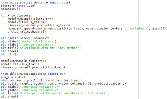
Because the GapMinder dataset only contain 56 available samples for all clustering variables, this dataset isn’t be split. A series of k-means cluster analyses were conducted on the training data specifying k=1-9 clusters, using Euclidean distance. The average distance from observations from the cluster centroid was plotted for each of the nine cluster solutions in an elbow curve to provide guidance for choosing the number of clusters to interpret.

Elbow curve of average distance from observations from the cluster centroid for the nine cluster solutions is as follows:

The elbow curve was inconclusive, suggesting that the 2, 3, 7 and 8-cluster solutions might be interpreted. The results below are for an interpretation of the 3-cluster solution.

Canonical discriminant analyses was used to reduce the 11 clustering variable down a few variables that accounted for most of the variance in the clustering variables.Following is the plot of the first two canonical variables for the clustering variables by cluster.

The above figure reveal the three clusters are almost perfectly divided, indicating the 3-cluster solution is a good solution. The outliers indicates that even if the split may be proper into there might be problems in later work on a proper model.

The means on the clustering variables showed that cluster 0 had the highest level of incomeperperson, breastcancerper100th, femaleemployrate, internet use rate, life expectation, oil consumption per person, polityscore, residual electric consumption per person, employ rate and urban rate which means the countries in cluster 0 may be high income and developed countries. Comparing cluster1 and two reveals that the countries in cluster 1 has higher incomeperperson, alcconsumption, femaleemplyrate, internetuserate, lifeexpectancy, polityscore, reelectricperperson, suicideper100th, employrate and urbanrate. Probably is the countries in cluster 1 more developed than in cluster 2. This conclusion can be confirmed by the average income per person of each cluster in following figure.

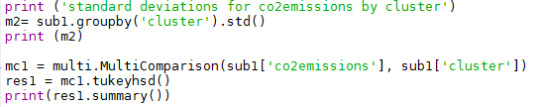
A tukey test, see below, was used for post hoc comparisons between the clusters. Results indicated differences between the clusters on co2emissions is insignificant. The CO2-emissions in cluster 0 (mean 3.3*10^10, std 7.7*10^10) is not on on 5 % significance level different from cluster 1 ( mean 9.4*10^9, std 1.0*10^10) and cluster 2 (mean 7.7*10^9, std 8.9*10^9).

[edeskar-dai-blog]

Assignement 3 - Run a lasso regression model

A lasso regression analysis was conducted to identify the most important  subset of variables to predict the quantitative response variable “CO2 emissions per capita” in the Gapminder dara set. The total number of predictor variables in the analysis is 14, all of them quantitative. The quantitative predictor variables are alcconsumption, armedforcesrate, breastcancerper100th, co2emissions, femaleemployrate, hivrate, internetuserate, lifeexpectancy, oilperperson, polityscore, relectricperperson, suicideper100th, employrate and urbanite. All predictor variables were standardized to have a mean of zero and a standard deviation of one in the analysis.

The python code used for the analysis:

Data were randomly split into a training set that included 80% of the observations (N=44) and a test set that included 20% of the observations (N=12). The least angle regression algorithm with k=10 fold cross validation was used to estimate the lasso regression model in the training set, and the model was validated using the test set. The change in the cross validation average (mean) squared error at each step was used to identify the best subset of predictor variables.

Following are the coefficient progression and mean square error for each fold of the model.

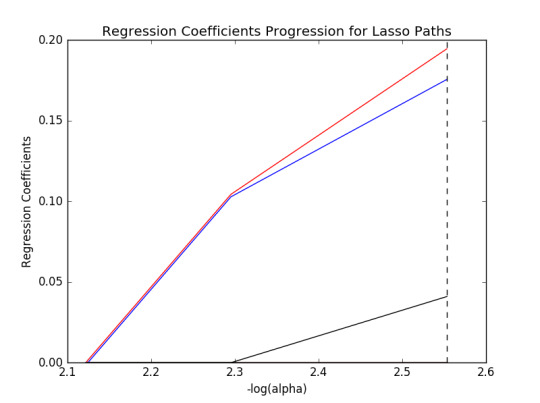
As expected, coefficients shrink to zero and mean square error for each fold increase as -log(alpha) decrease(This means alpha increase and the more coefficients will shrink to zero and the model will be simpler).

The output from the analysis is shown below. 

The dictionary of regressions coefficients of the  14 predictor variables shows that 3 were retained in the selected model; urbanrate (0.007), incomeperperson (0.029) and armedforcerate (0.028). Incomeperperson and armedforcerate  .are the two most important predictor varaibles and are equally important according to the results. But the regressions coefficients are low for all of the three remaining predictor variables. These three variables explaines about 60 % of the varaibility in the model.

The mean square error on test set is much higher compared to the training set. The R-square is similar for the test and training on test set is much lower than train set. The result indicates that  the selected model is pretty good even if the data set only contains  56 samples.  But the selected variables is not expected and thus should not the model be automatically trusted.

[edeskar-dai-blog]

Assignment 2: Run a random forest

A random forest analysis are method used to evaluate the importance of a series of explanatory variables in predicting a binary categorical response variable. Here has the Gapminder data set been used. The response variable CO2-emissions per capita has been computed based on the oil consumption per capita. The CO2-emission per capita variable has been splitted into two categories, low and high, by splitting the variable at its mean value.

The code used for the analysis:

The result below ranks the importance in all explanatory variables included in the decision tree. The three most important response variables were lifeexpectancy, internetuserate and breastcancerper100th. The accuracy was 91 % for this model, The high accuracy is probably due to small size of the  dataset, 56 samples.

A random forest from 1 to 25 decision trees were grown to evaluate if more trees are contributing to the model. The accuracy of the sets of trees as a function of the number of trees are displayed below.

Since the accuracy flips as the forest grows and increases the interpretation is that a single decision tree is the most appropriate model.

Summary

The 3 most important variables, identified by the decision tree for explanatory variable CO2-emissions per capita were life expectancy, internet use rate and breastcancer per 100th persons. This result is not expected. The analysis of the effect of growing the number of trees in the model by a random forest shows that one tree is appropriate to model the CO2-emissions per capita.

[edeskar-dai-blog]

Assignment 1 - Run a decision tree

Decision tree analysis was performed to test nonlinear relationships among a series of explanatory variables and a binary, categorical response variable on the gapminder dataset. The algorithm tests all possible separations (categorical) or cut points (quantitative).

As response variable co2_dummy has been used. The variable has been created by computing the CO2-emissions per person based on the variable oilperperson and conversion factors to CO2-emissions (the co2emission variable in the gapminder dataset is the accumulated CO2-emissions). The co2_dummy variable were created by splitting the computed CO2-emissions by the mean. 0 indicates that the country has CO2-emissions lower than the average and 1 above the average.

The python code used were:

The variables oilperperson and co2percapia was dropped for the analysis since they both were used to create the response variable co2_dummy. The remaining explanatory variables and the response variable are shown below.

The accuracy score was calculated for all the combinations of explanatory variables vs the response variable. As seen below the accuracy coefficient was 1.0 for several  combinations. This is not a suprice since the sample size is very low, 56. A low sample size makes it easier for the model to find a valid split for all combinations.

One of the decision trees-medel and the incorprated variables are displayed below. It is based on three response variables reelectricperperson (X7), internetuserrate (X4) and alcconcumption  (X0). The response (target) variable is co2_dummy, < = 0.5 means low CO2-emissions and > 0.5 high CO2-emissions.

The interpretation of the decision tree is that a country with use of residential relectricity less than about 1450 kWh per person (24 of totally 33 countries) and has an internet user rate less than about 75 %, 23 of the subset of 24 countries,  has low CO2-emissions per capita. If the internet user rate is above 75 % of the subset 1 of the 24 has high CO2-emissions. The other branch of the tree, where the use of residential electricity is higher than about 1450 kWh, 9 of totally 33 countries, the second split is based on alcohol consumption. If the country has an alcohol consumption less than 12 l alcohol per person 8 of 9 countries of this subset has high CO2-emissions per capita. If the alcohol consumption is higher than 12 l per person and year 1 of the subset of 9 countries has low CO2-emissions.

This model is probably not the best model to predict CO2-emissions among all the possible combinations of variables.

[edeskar-dai-blog]

Machine learning course

[edeskar-dai-blog]

Assignment 4 logistic regression

In this asignment I use the Gapminder data set. The response variable is in CO2-emissions per person. CO2-emission per person is computed by oil consumptiion per person.  It’s a quantitative variable and has been binned into two categories(by splitting at the mean value) to create a new binary response variable CO2_dummy which indicates if the nation releases more or less CO2 than average or not..The explanatory variable is urbanrate and the potential explanatory variable is residential use of electricity per person. The hypthesis is urbanisation leads to less CO2-emissions (in favour for use of electricity as energy source).

After binning the 39 observation belongs to category 0 and 22 to category 1.

The basic regression models uses CO2-emissions per person as response variable and urbanrate as quantitative explanatory variable.

The regression analysis shows that the relation between CO2-emissions per person and urbanrate is significant (p=0.001). The odd ratio is low but positive, OR = 1.09. The 95 % confidence interval for OR is 1.03-1.14.

Adding the variable residential use of electricity per person (el) to the regression model shows that el is an confounding variable. Urbanrate is not longer statistical significant (p=0.225). The confounding varaible el is statistical sigificant (p=0.001), the odds ratio OR = 1.0 an the 95 % confidence interval for OR is 1.0 - 1.01.

The income per person was also tested as confounding variable to urbanrate. When adding income the urbanrat is no longer statistical significant (p=0.591). Income per person is statistical significant (p<0.0001) and is thus a confounding variable. OR for income per person is 1.0 and the 95 % confidence interval is 1.0-1.0

The conclusion is that categorising CO2-emission per person into to a two level categorical response variable is a bad idea when running a logistic regression by using urbanrate, electrical use per person and income per person as explanatory variables. Both electrical use per person and income per person is confounding variables to urbanrate in the models. But the oddsratio for these confounding variables are 1 respectively. Thus does they not add any more explanations to the models. The conclusion is that the 0-hypothesis holds. No valid relation can be found between the CO2-emissions per person as response variable and urbanrate, residential use of electricity and income as explanatory variables.

[edeskar-dai-blog]

Assignment 3 - Test a multiple regression analysis

The main hypothesis is that there is a relationship between urbanrate and CO2-emissions and that a high urbanrate contrubutes toward a shift of use of electricity.

The analysis focus on the relationship bewteen urban rate (explanatory variable) and CO2-emissions (dependent variable). The following variables are investigates as explanatory variables if they are reasonable to add in a multiple regression prediction model:

The residential use of electricity 

The income rate

Oil consumption per person

Ratio (residential use of electricity / oil consumption)

The first step is to investigate if the relationship in between the urban rate (explanatory variable) and CO2-emissions (dependent variable) is linerar or ploynomial. In the figure below both a linear regression line and a second order polynomial model are compared.

The scatterplott shows a better prediction for the polynomial model compared to the linear, especialy at low and high urbanrates. Some outliers, especially at high urbanrates are not captured by either of the models.

The output of the linear and polynomial regression analysis are shown below.

The prediction  model for the linear regression model is:

CO2-emissions per person = 0.063 + 0.0022 * urbanrate

The prediction  model for the quadratic regression model is:

CO2-emissions  per person= 0.0435 + 0.0027 * urbanrate + 5.877e-5*urbanrate^2

Both the linear model and both terms of the quadratic regression model are statistic significant (p<0.0001), all coefficients positive and non of the reported confidence intervals includes 0 . The quadratic models has a higher r2-value (0.335) compared to the linear model (0.249) and is thus a better prediction model for the CO2-emissions. From here the quadratic model is used.

All possible confounding variables, previously in the courses,  was added to the quadratic regression model in order to check in they are statistically significant or confounding to the model.The added explanatory variables after centering were income per persons, oil consumption per person, residential electricity per person and ratio (residential electricity / oil per person). The r-square value for the model is 1.0 which means that the model is either perfect or that the explanatory variables are not independent at all in relation to the the dependent variable. The regression results shows that both urban rate (p-value = 0.966, confidence interval [-6.35e-17, 6.09e-17]) and the quadratic term  of urban rate (p-value = 0.915, confidence interval [-2.05e-18, 2.28e-18]) are not longer statistical significant. The income per person is also not a significant in the regression analysis (p=0.213, confidence interval [-1.43e-19, 3.26 e-20). In this model are oil consumption per person, residential electricity per person and ratio (residential electricity / oil per person confounding variables. 

The beta and p-values for all explanatory variables in the regression model are:

Urbanrate (urb_c) - Beta = -1.238e-18, p =0.966

urb_c^2  - Beta = -1.16e-19, p < 0.0001

Ratio resedential electricity / oil consumption) (ratio_c)   - Beta = -4.923e-18, p < 0.0001

Residential electricity (el_c)   - Beta = -1.389e-18, p < 0.0001

Oil consumption (oil_c)   - Beta = 0.0432, p < 0.0001

Income (income_c)   - Beta = -5.06e-20, p =0.213

In normal cases should the non-significant variables be rejected and the confounding variables should be further investigated. But in this case is the dependent variable computed based on the variable oil per person. Oil per person is also used to compute the varaible ratio. These variable are not independent in relation to the dependent variables and are violation the basic assumptions of the analysis. Based on lack of independence are all of these variables discarded and another regression analysis including the urban rate, the quadratic term of urban rate, residential electricity per person and income per person. The new model has a r-square value of 0.442 which is higher than the quadric model for urban rate (0.335). But none of the added explanatory variables are statistical significant or the confidence intervals excluding 0. These are excluded from the model.

After rejecting the additional explanatory variables the choice is to keep the quadratic urbanrate model, previous defined as:

CO2-emissions  per person= 0.0435 + 0.0027 * urbanrate + 5.877e-5*urbanrate^2  

The Q-Q plot below reveals that all lines does not follow  Normal distribution. An extreme outlier is found in the higher range. Around the center of the plot the residuals migrates from above the line to below the line. This indicates a heavy tailed distribution. A clear outlier at the right upper corner in the plot is identified.

The standardised residual plot for the quadratic model of urbanrate vs CO2-emissions fulfils the requrements of 68 % of the residuals being in [-1,1] and 95 % in the inteval [-2.2]. 1 outlier at 5.5 standard deviations is identified. It is equal to 1.5 % and is by role of thumb not indicating poor model fit but should be looked at closer. Adding more explanatory results has not worked since they have eiher not been independent or contributed statisticall significant to the explanatory model.

In the regressionplots below the outlier found  in the residual plot is clearly visible in all of the plots. The rsidual pots (upper right) shows an increase in in the variance of the residuals, a funnel shape. The partial regression plot shows an sinus-shaped pattern. The information from these plots indicates that the requirement of linearity may not be met.

The leverage plot reveals that it is point number 173 that is the extreme outlier. It has a a high effect on the model due to high standard deviation an relatively high leverage. The other outliers has comparable low impact since these datat points are within two standard deviations.

The result of this analysis is that the hypothesis that urbanrate increases the CO2-emissions is valid. However, int can to be concluded that higher urbanrate contributes toward a shift of more use of residential electricity.

The overall conclusion is that the quadratic model of urbanrate without adding more variables is the most reasonable model. There are signs that the model does not fulfil the assumptions of a valid model. The prediction model shows a positive ralationship in between urban rate and CO2-emissions. The model explains 33.5 % of the variablitiy. The prediction models is:

CO2-emissions  per person= 0.0435 + 0.0027 * urbanrate + 5.877e-5*urbanrate^2

[edeskar-dai-blog]

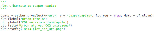
Assignment 2 - Basic linear regression analysis

A basic linear regressions analysis has been performed on the explanatory variable ‘Urbanrate’ (%)and the computed response variable ���CO2-emissions per capita’ (ton/person) from the GapMinder dataset.

The code used to perform the analysis in Python is presented below:

Import the necessary modules:

Import the data from the GapMinder dataset:

Subset the dataframe to the varaiables of interest. All variables used to cover the aoverall research questions are included:

Recode the variables:

Convert the data in the dataframe to numeric. The old code is used since the new, preferred code does not work on my system:

Compute the response varaible “CO2 emissions per Capita” (tons/person) based on the oil consumption.:

Perform the regression analysis and generate a scatterplot:

Code fore centering explanatory variable and check if the centering was successful. The new centered variable is called ‘urb_centered’

The result of the centerin the expanatory variable is shown below. The centered variable has not been used in the latter regresion analyis. The centering was successful since ‘urb_centered’ = 0.

The regressions result and regression plot are shown below:

The regression analysis are based on two quantitative variables; “Urbanrate” as explanatory variable and “CO2 emission per capita” as dependend variable.

n the analysis “Urbanrate” only 62 observations of totaly 213 in the imported data-set are included in the regresion analysis and scatter plot. There is a lot of empty observations in the variable ‘oilconsumption’ used to compute the “CO2-emissions per capita”. The R-square paramete indicates that the regression model explains 28.3 % of variability in the model which relatively low. The probility based on F-statistic is far below 0,005 (8.52 E-06) which means that the variables are correlated on a statistical significant level.

The linear regression analysis prediction model of the relationship between the dependent variale and response variable is:

 “CO2 emissions per capita” = -0.1065 + 0.024* “Urbanrate”.

The P-value for the relation between the explanatory variable and the dependent variable is < 0.0001.

Some of the basic assumptions for linear regression can be checked by looking at he scatter plot. The assumption of a linear relationship in between the variables is not perfect since the variability of the data increases at the higher ranges of the explanatory variable. It also means that the criteria for homoscedasticty is not met. The scatterplot shows that there are outliers, especially in the higher range of Urbanisation rate that influence the linear regression model. The outliers indicates that a non-linear model may should be tested or that these data points needs to be evaluated separatly if the should be included in the analysis or not.

The overal conclusion is that CO2-emissions is positivley correlated to urbanisation, i.e. the more people living in urban areas - the more CO2-emissions. Even if the relationship is statistically significant only 28.3 % of the variability is explained by the linear regression model. It is possible that more variables added to the model can increase the explanation of variability or change the the regression model to e.g. polynomial.

[edeskar-dai-blog]

Assignment 1 - Writing about your data

Sample (step 1) The sample is provided by the Gapminder foundation, a non-profit organisation, promoting sustainable global development and achievmenent of the United Nations Millenium Development Goals. The Gapminder Foundation compiles statistics on indicators of status and development in the areas of economy, environment, health, education and social aspects for all countries. The sample (n=213) comprises all official countries in the UN and (193) and twenty additional regions of special status from a historical perspective, e.g. Hong-Kong. 

(NB! Here is the sample (n=213) based on the number of observations in the data set file provided in the course. The provided codebook in the course states n=215 which is incorrect)

Procedure (step 2)

The data collected by the Gapminder foundation is provided by a range of official organisations ( e.g. the World Bank and UN organisations), interest organisations (e.g. International Labor Organization), companies ranking (e.g. Forbes), some reseach reports/papers and own work by the Gapminder foundation. The Gapminder foundation serves as a portal to access the data for analysis by the organisations owns tools or for anybody to explore.

Measures (step 3)

The effect of urbanisation ��on greenhouse emissions was assessed by analysis of the urbanrate, oil consumption per capita and use of residential electricity. The oil consumption was used to quantify the carbon dioxide emissions and the ratio (coded as ratio) between the use of residiential electricity and oil consumption as an indicator of changes in use of energy sources.

Urbanrate, the explanatory variable, (coded as urbanrate) was based on the World bank data for 2008 urban population (% of total population). Urban population refers to people living in urban areas as defined by national statistical offices (calculated using World Bank population estimates and urban ratios from the United Nations World Urbanization Prospects). Urbanrate ranges from 0-100 %There are 203 observations of urbanrate in the dataset.

The oil consumption,  response variable, (coded as oilperperson) is the reported oil consumption per capita (tonnes per person) for 2010  by BP. The oil consumption are recalculated to carbon dioxide emissions by assuming that one barrel of oil releases 317 kg of carbon dioxide and that one ton oil equals 7.33 barrels, figures used by the IPPC. Oil consumption per capita ranges from 0.03-12.2 tonnes oil per person equivalent to 0.01-0.52 tonnes of carbon dioxide per person. The dataset of oil per person contains 63 observations. 

As indicator of the use of electricity (coded as reelectric)the residential use of electricity per person (kWh/person) for 2008 resported by the International Energy Agency was used to calculate the response variable ratio. Residential electricity ranges from 0-11154 kwh/person and has 144 observations in the dataset.

[edeskar-dai-blog]

Assignment 4

In assignment 4 the effect of the moderationg variable “Income per person” is studied on the relation between “Urban rate” and “CO2 emissions per capita. The analysis is based on the Gapminder dataset.

“CO2 emissions per capita” is created by a re-calculating the variable “oilperperson” to CO2 emissions.

A scatterplot, including a linear regression line was created for occular inspection of the data urbanrate vs. CO2- emissions per capita.

As seen in the plot there seems to be a positive linear relationship between the “Urban rate”and “CO2 emissions per capita”.

The Pearson correlation coefficient was computed for “Urban rate” vs. .”CO2-emissions per capita”:

The Pearson correlation coefficient shows a positive linear correlation (r=0.499) and the relation is stasticially significant at a high level, p = 4.18e-05. 

“Income per person” has been tested as moderating variable. The moderating variable was divided into three classes (LOW, MIDDLE, HIGH) by the following code:

The number of observervations in each group are LOW =20, MIDDLE= 15, HIGH=26.

A Pearson correlation test was done for each class of the moderating variable “Income per person”:

The following scatter plots visualizes the subset of the moderating variables:

Significant correlation by adding the moderating variable “Income per person” where LOW (p-value=0.027) and HIGH (p-value)=0.026). The association (Persson coefficient) are approximatley equal betwen the analysis not including the moderationg variable and the LOW category of the moderating. The HIGH category shows a slightly lower positive linear Pearson correlation (0.43) compared to the original analysis (0.499).

The conclusion is that adding the moderate varaible “Income per person” does not improve the interpretation of the relation between “Urbanrate” and “CO2-emission per capita”. Adding the moderating variable increases the p-value and thus is negative from a statistical significancy point of view. Considering the results from the moderating variable is in the mid-range of “Income per person” that deviate from the result in the original analysis.

[edeskar-dai-blog]

Assignment 3

In assignment 3 the varaibles urbanrate vs. the ratio of use of residential electricity and oil per capita form the Gapminder Dataset by Pearson correlation. The studied question is if the urban rate effects the us of energy source. An increase in the response variable the ratio of use of residential electricity and oil per capita indicates a releatively higher use of electricty as energy source compared to oil.

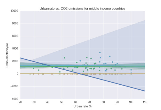
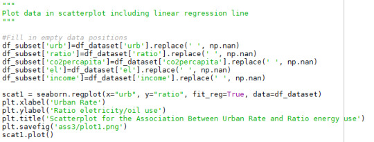
The first step is to visualise the data in a scatter-plot. In this plot has the linear regression line has been included.

The code for generating the scatterplot is:

The generated plot:

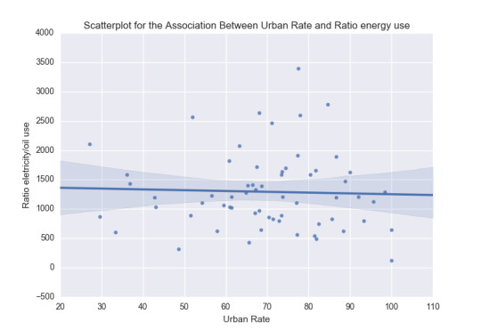
The plot indicates a very weak negative relation between urbanrate vs. the ratio of use of residential electricity and oil per capita. The majority of the datapoints are positioned in the range of approximatly 60-90 % urbanrate and shows a high variability.

A linear Pearson correlation test was performed on the variables in the scatter plot. The used code is shown below:

The result of the linear Pearson correlation test is:

The result confirmes the observations of the scatter plot. The linear Pearson coefficient r = -0.0371 shows a low negative linear correlation between the explanatory and response variable. The p-value, p = 0.776, is higher than p = 0.05 and thus is the relation between the variables not statistical significant.

The conclusion is that no linear correlation between the variables urbanrate vs. the ratio of use of residential electricity and oil per capita on a statistical significant level. The energy mix is not linear correlated with the urban rate according to this dataset.

[edeskar-dai-blog]

Assignment 2

In assignment 2 a chi-square test of independence has been applied on the Gapminder dataset in order to test if the energy mix used is dependent of people living in cities or not.

The data analysis has been performed on the Gapminder data-set. As explanatory variable has urban rate, i.e. the percentage of the population living in urban areas, neen used. The urban rate has been binned into quartiles in order to be represented as a categorical variable. The energy mix are expressed as the ration between the use of resdential electricity (kWh) per capita and the oil consumption per capita (ton). The ratio has been converted into a 2-level categorial variable by arbitary assuming that a low level of ratio, i.e high amount of oil is < 2000, and a high amount of use of electricity is > 2000 based on occular inspection of the frequency distribution of the dependendent variable ratio.

The hypothesis is:

0-Hypothesis: The ratio of electricty/oil consumption equal for all urbanrates

Alternate Hypothesis: The ratio electricty/oil consumption is not equal for all urbanrates

The hypothesis is tested at p=0.05.

The code for running the Chi-square test (from creating the variable ratio):

The analysed data is visualised below:

The result from the analysis is shown below:

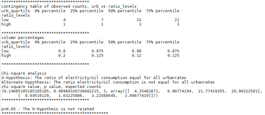
The alternate hypothesis is rejected since the p-value > 0.05. Thus are the energy mix considered to be equal for the different urban rates in the dataset.

A Post Hoc-analysis has been performed on all combinations of the expanatory variables. The Bonferroni probability has been used as p-value, here 0.083 has been used to judge if the combination can reject the 0-hypothesis wiithout cause a Type 1 error The code is shown below:

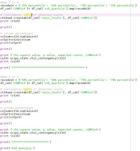
The result from the pos-hoc analysis is shown below:

No combination has a p-value < 0.0083. None of the categories could reject the 0-hypothesis.

The conclusion of the chi-square tests is that there are no difference in the energy mix (ratio of the use of electricty and oil) between countries of different degrees of urbanisation based on 5 % significance level.

[edeskar-dai-blog]

Assignment 1

The research questions are if the urbansisation increases the CO2-emissions and if urbanisation is increasing the use of electricity in favour of oil.

In this analysis the urbanrate (explanatory variable) has ben converted to an categorical variabel by divide it into quartiles (four categories). ANOVA analysis has been perfomed on urbanrate vs CO2-emission and urbanrate vs ratio of electricity use and oil use. The response variables CO2-emissions and ratio of electricity use/oil consumption are quantitative.

ANOVA of urbanrate vs CO2-emissions

0-hypothesis: There are no difference in between the levels of urbanrate and CO2-emissions.

Alternate Hypothesis: There is a significant difference in the mean CO2-emissions in between the different quartiles of urbanrate.

Code:

ANOVA results:

Post-hoc analysis:

The ANOVA-analysis shows that there are no significant difference in between the categorized urban rate quartiles and CO2-emissions (prob = 0.30 > 0.05). The 0-hypothesis is not rejected. However, the fourth quartiles shows that there are a difference in CO2-emission for this category compared to the others.

The Post-hoc analysis shows that all four quartiles are rejected by the Tukey’s test. Thus is also the indicated difference for the fourth quartile of urban rate also rejected. The test show no significant difference between the quartiles of urban rate and CO2-emissions.

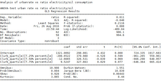
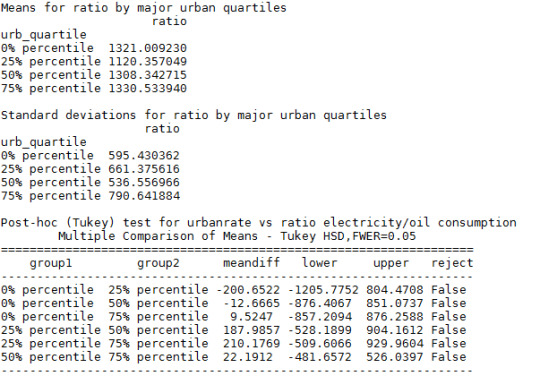
ANOVA of urbanrate vs ratio electricity/oil consumption

0-Hypothesis: There are no difference in between the levels of urbanrate and ratio of electricity use/oil consumption.

Alternate Hypothesis: There is a significant difference in the use of electricty relative the use of oil between the different quartiles of urbanrate.

Code:

ANOVA:

Post-hoc:

The ANOVA-analysis shows that there are no significant difference in between the categorized urban rate quartiles and ratio of electricity use/oil consumption (prob = 0.211 > 0.05). The 0-hypothesis is not rejected.

The Post-hoc analysis shows that all four quartiles are rejected by the Tukey’s test.

The tests shows no difference in between the levels of urbanrate and ratio of electricity use/oil consumption

[edeskar-dai-blog]

Data analysis tools

Here are the assignments in the second course presented.

The dataset used is the GapMinder dataset. The research questions:

Does the urbanisation increase the CO2-emissions?

Does the urbanisation favor the use of electricity over oil as energy source?