editukas-blog1

[editukas-blog1]

Methods Section, Milestone Assignment 2

Dear colleagues students, 

let me present 2nd part of capstone project. I changed my plan for working with World Bank Data and for my final project chose dataset from one of DrivenData competitions - prediction of H1N1 and seasonal flu vaccines.

Sample

The sample includes N=26706 respondent answers to the phone survey, which was conducted in 2009-2010 in United States (National 2009 H1N1 Flu Survey). Respondents were asked whether they had received the H1N1 and seasonal flu vaccines, also some questions about themselves.

Measures

In this data set, there are two response variables, 1) showing whether respondent received H1N1 flu vaccine, 2) whether respondent received seasonal flu vaccine. Both are binary variables. Some respondents didn't get either vaccine, others got only one, and some got both.

There are 2 groups of predictors: behavioral and personal situation.

Behavior /opinions describing variables: level of concern about the H1N1, level of knowledge about H1N1, has taken antiviral medications (yes/no), has avoided close contact with others with flu-like symptoms (yes/no), has bought a face mask (yes/no), has frequently washed hands or used hand sanitizer (yes/no), has reduced time at large gatherings (yes/no), has reduced contact with people outside of own household (yes/no), has avoided touching eyes, nose, or mouth (yes/no), H1N1 flu vaccine was recommended by doctor (yes/no), seasonal flu vaccine was recommended by doctor (yes/no), has any of the chronic medical conditions (yes/no), has regular close contact with a child under the age of six months (yes/no), is a healthcare worker (yes/no), has health insurance (yes/no), respondent's opinion about H1N1 vaccine effectiveness (1 „not at all effective“ to 5 „very effective“), respondent's opinion about risk of getting sick with H1N1 flu without vaccine (1 „very low“ to 5 „very high“), respondent's worry of getting sick from taking H1N1 vaccine (1 „not at all worried“ to 5 „very worried“), respondent's opinion about seasonal flu vaccine effectiveness (1 „not at all effective“ to 5 „very effective“), respondent's opinion about risk of getting sick with seasonal flu without vaccine (1 „very low“ to 5 „very high“), respondent's worry of getting sick from taking seasonal flu vaccine (1 „not at all worried“ to 5 „very worried“).

Personal situation describing variables: age, race, sex, education level, marital status, household income, number of aduls in household, number of children in household, housing situation, employment status, type of industry, type of occupation, respondents residence, residence in metropolitan statistical areas.

Each row in the dataset represents one person who responded to the National 2009 H1N1 Flu Survey.

Analyses

For descriptive analysis, the distributions for the predictors and response variables: H1N1 and seasonal flu vaccines, were evaluated by examining frequency tables for categorical variables and calculating the mean, standard deviation and minimum and maximum values for quantitative variables.

For bivariate analysis, logistic regression method was used to test bivariate associations between chosen behavioral/opinions predictors and both response variables, the H1N1 and seasonal flu vaccines.

Lastly, multivariate multiple linear regression analysis was performed. Each dependent variable was separately regressed on the predictors. All predictor variables were standardized to have a mean=0 and standard deviation=1 prior to conducting the multivariate multiple linear regression analysis.  For cross-validation testing to avoid overfitting graphical residual analysis was performed.to consider the fit, predicted values were put on the x axis and the estimated residuals on the y axis.

Please review my work and let me know what you think.

Sincerely,

Edita

[editukas-blog1]

Title and Introduction to the Research Question, Milestone Assignment 1

Dear colleagues students,

for my final project in Data Analysis and Interpretation specialization I chose the following topic:

The Association between Countries’ Demographic & Financial Wealth Factors

The purpose of this study was to identify which demographic factors such as life expectancy at birth, infant mortality rate, net migration, population ages 65 and above, birth rate are most strongly associated with countries’ financial wealth factors, such as GDP per capita and health expenditure per capita.

As a data analysis student, I am passionate about working with important data and understanding what it shows. I chose World Bank data set to work with. I’m expecting that this research will allow me to make some predictions from demographic factors what could be certain country’s financial wealth level.

Please review my work. Thank you.

Sincerely,

Edita

[editukas-blog1]

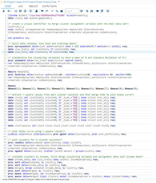
K-means Cluster Analysis, 4.4 assignment

Dear colleagues students,

I performed a K-means cluster analysis was for gap minder data set to identify whether by analyzing 9 clustering variables it would be possible to predict income per person in different countries. Clustering variables:

femaleemployrate 

employrate 

Internetuserate

lifeexpectancy 

polityscore 

relectricperperson 

urbanrate 

oilperperson 

co2emissions

 All clustering variables were quantitative and standardized to have a mean of 0 and a standard deviation of 1.

Data were randomly split into a training set that included 70% of the observations (N=150) and a test set that included 30% of the observations (N=64). 

Elbow curve of r-square values for the 9 cluster solutions  suggests that the 3, 4, 6, 7 and 8-cluster solutions might be interpreted (most prominent bends).

The results below are for an interpretation of the 4-cluster solution.

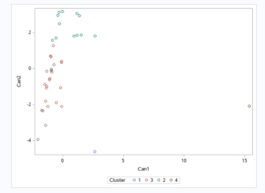
Canonical discriminant analyses was used to reduce the 9 clustering variable down a few variables that accounted for most of the variance in the clustering variables. A scatterplot of the first two canonical variables by cluster indicated that the observations in clusters 3 and 2 were more densely packed and more numerous and did not overlap very much with the other clusters. Cluster 4 was generally distinct, with only a few observations. Observations in cluster 1 were spread out more than the other clusters, showing higher cluster variance than in others. The results of this plot suggest that the best cluster solution may have fewer than 4 clusters. Also, data set is relatively small, so it would be important to also evaluate the cluster solutions with fewer than 4 clusters (spoiler alert - when data is not split into training and test sets, 3-cluster solution explains differences better, I checked this afterwards).

Plot of the first two canonical variables for the clustering variables by cluster.  

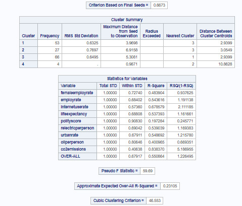
The means on the clustering variables showed that, compared to the other clusters, countries in cluster 1 have highest female and overall employment rates compared to others, but lowest internet usage, urbanization, life expectancy, oil and electricity usage, democracy scores and co2 emission rates. We can safely predict this would be the cluster of countries with lowest income per person.

Cluster 4 countries have 2nd highest female and overall employment rates and life expectancy compared to others, and highest (with big difference from other clusters) internet usage, urbanization, oil and electricity usage, democracy scores and co2 emission rates. We can predict this would be the cluster of countries with highest income per person.

Clusters 3 and 2 have big distinction among them by all parameters, and cluster 2 countries clearly being more developed and of higher personal income than cluster 3 .

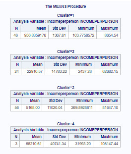
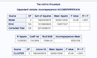
ANOVA procedure was performed to test for significant differences between the clusters on income per person. A tukey test was used for post hoc comparisons between the clusters. Results indicate significant differences between the clusters on income (F=43.09, p<.0001). The tukey post hoc comparisons showes significant differences between clusters on income, with the exception that clusters 1 and 3 were not significantly different from each other.  Countries in cluster 4 had the highest income per person rate (mean=58210.61, sd=40741.34), and cluster 1 countries had the lowest income per person (mean=956.84, sd=1367.61). This model explains 51% of observations (R-square=0.5083).

Please review my work. Thank you!

Sincerely,

Edita

[editukas-blog1]

Running a Lasso Regression Analysis, 4.3 assignment

Dear colleagues students,

I performed lasso regression analysis to identify a subset of 11 categorical and quantitative predictor variables that best predict a quantitative response variable measuring personal income of participants. 

Categorical predictors included gender, major depression, general anxiety, tobacco dependency, gambling problems, working situation (if working full day or not), race (white or other race). Quantitative predictor variables include age, educational degree, marital status, alcohol problems. 

Here’s program code:

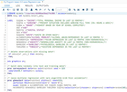
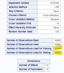
Data were randomly split into a training set that included 70% of the observations (N=30166) and a test set that included 30% of the observations (N=12927). 

The least angle regression algorithm with k=10 fold cross validation was used to estimate the lasso regression model in the training set, and the model was validated using the test set. 

The change in the cross validation average squared error at each step was used to identify the best subset of predictor variables.

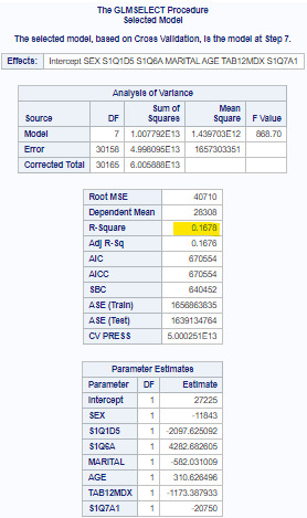
Of the 11 predictor variables, 7 were retained in the selected model. During the estimation process, educational degree, working situation (full time or not) and sex were most strongly associated with current personal income, followed by age, marital status, race and tobacco dependency. 

These 7 variables accounted for 16.8% of the variance in the personal income response variable.

Please review my work, thank you!

Sincerely,

Edita

[editukas-blog1]

Random Forests, 4.2 assignment

Dear colleagues students,

Here’s my code for random forest building.

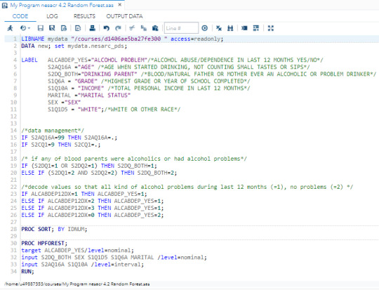
Random forest analysis was performed to evaluate the importance of a series of explanatory variables in predicting a binary, categorical response variable. The following explanatory variables were included as possible contributors to a random forest evaluating participants, who had alcohol problems in last 12 months (ALABDEP_YES response variable) :

S2AQ16A ="Age" (age when started drinking, not counting small tastes or sips)

S2DQ_BOTH="Drinking Parent" (blood/natural father or mother ever an alcoholic or problem drinker)

S1Q6A = "Grade" (highest grade or year of school completed)

S1Q10A = "Income" (total personal income in last 12 months)

MARITAL ="Marital Status"

SEX ="Sex"

S1Q1D5 = "White" (white or other race)

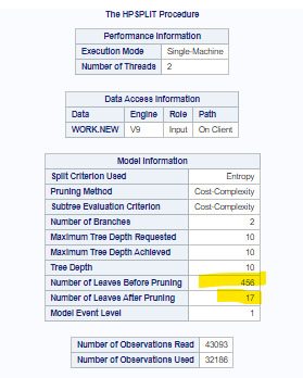
Fit statistics, first and last 10 trees:

The accuracy of the random forest is 92%, and this average square error rate (OOB) slightly goes down, improving overall accuracy of the model.

Variables ranked by importance:

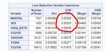
From seven variables represented here, Gini column is negative for 4 variables, and the OOB margin column is negative for 1. We can say that explanatory variables with the highest relative importance scores were marital status, sex of participants and having at least one drinking parent.

Please review my work, thank you!

Sincerely,

Edita

[editukas-blog1]

Running a Classification Tree, 4.1 assignment

Dear colleagues students,

I performed  decision tree analysis to test nonlinear relationships among a series of explanatory variables and a binary categorical response variable.

The following explanatory variables were included as possible contributors to a classification tree model evaluating participants, who had alcohol problems in last 12 months (ALABDEP_YES response variable) :

S2AQ16A ="Age" (age when started drinking, not counting small tastes or sips)

S2DQ_BOTH="Drinking Parent" (blood/natural father or mother ever an alcoholic or problem drinker)

S1Q6A = "Grade" (highest grade or year of school completed)

S1Q10A = "Income" (total personal income in last 12 months)

MARITAL ="Marital Status"

SEX ="Sex"

S1Q1D5 = "White" (white or other race)

Variables ranked by importance:

Age when started drinking was the first variable to separate the sample into two subgroups. Those who started drinking earlier than 17.48 years, are more likely to experience current drinking problems than those who started >=17.48 years (17% vs. 6.4%).

Second subdivision is made by variable “marital status”. Those who are “married” (=1) or “widowed” (=3) are less likely to experience drinking problems than those who are divorced, separated, were never married or living together  (10.4% vs. 24.3%).

Of group mentioned above, 3rd division is made by sex, and men are more likely to experience alcohol related problems than women (29.8% vs. 17.9%).

However, this model classified correctly only 0.35% of sample for those who have current drinking problems (sensitivity) and 99.99% of those who don’t have such problems (specificity).

Please review my work, thank you.

Sincerely,

Edita

[editukas-blog1]

Test a Logistic Regression Model, 4th week assignment

Dear colleagues students,

Here is my logistic regression analysis for this week assignment.

Code:

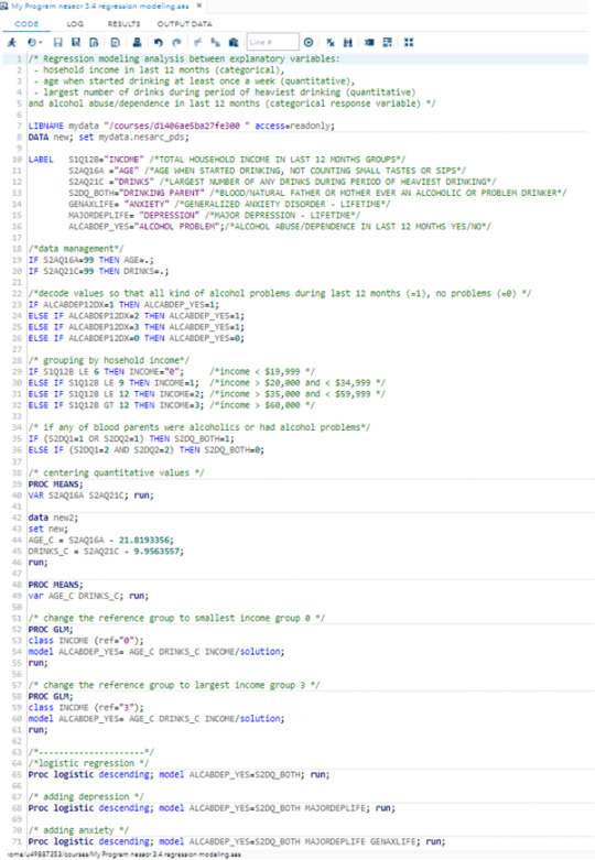
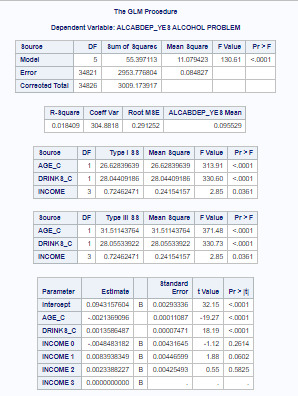
I was trying to prove if my hypothesis is correct: age when started drinking ( primary explanatory variable) is associated with participant’s alcohol dependence. Other explanatory variables - largest number of drinks during periods of drinking and household income in last 12 months (collapsed into 4 groups by quartiles).

We can see significant association between drinking problems for participants and age when started drinking (p<.0001), largest number of drinks during periods of heaviest drinking (p<.0001) and household income group (p=.036).

In this model, household income group might be confounding variable as its addition weakens association between starting drinking age and current alcohol problems.

When income group to compare is “0″ (smallest income), then we can still see significant association between drinking problems for participants from this group compared to participants from group 1 (p=.004). There is no significant association  between drinking problems for participants from this group compared to participants from group 2 and 3 (p=.1 and p=.26).

When income group changed to “3″ we can no longer see significant association in between participants from this group drinking problems compared with participants from other income groups (all p >0.05).

Logistic Regression

The outputs from logistic regression model:

a) Only association between drinking parent (S2DQ_BOTH) and drinking problem (ALCABDEP_YES).

In this case  OR=2.12, 95% CI = 1.96-2.29, p<.0001.

b) with additional explanatory values major depression (MAJORDEPLIFE) and general anxiety (GENANXLIFE)

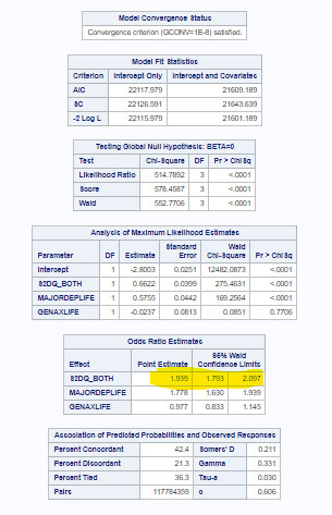
From logistical regression model we can suggest that in this analysis major depression and general anxiety are confounders to drinking parent (S2DQ_BOTH) variable.

After adjusting for confounders, we can say that persons having at least one drinking parent were almost 2 times more likely to have alcohol problems themselves than those participants whos’ parents didn’t drink (OR=1.94, 95% CI = 1.79-2.1, p<.0001). 

Please review my work. Thank you.

Sincerely,

Edita

[editukas-blog1]

Testing a Multiple Regression Model,  3rd week assignment

Dear colleagues students,

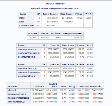
for regression modeling I chose data from gapminder dataset and decided to check if life expectancy is associated with income per person and alcohol consumption variables.

Income per person and alcohol consumption values were centered.

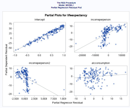
Here are required regression diagnostic plots:

a)  Q-q plot shows normal distribution of residuals, meaning that the error terms are normally distributed.

b) Standardized residuals for all observations. The standard deviation of the residuals calculates how much the data points spread around the regression line, we can see that most values fall in range between -2 and 2.

c) Leverage plot shows how far away the independent variable values of an observation are from those of the other observations. We can see several outliers and one high-leverage point which is at extreme value of the independent variable.

Conclusion of multiple regression is that income per person (Beta=.001, p<.0001) is significantly and positively associated with life expectancy. Alcohol consumption however was not significantly associated with life expectancy (Beta= 0.15, p=.1915). Both GLM and REG procedures show that alcohol consumption is a potential confounding variable.

This model explains pretty big part of sample data (R-square value is 0.47, that means 47% of data).

Please review my work.

Thank you in advance,

Edita

[editukas-blog1]

Testing a Basic Linear Regression Model, 2nd week assignment

Dear colleagues students,

for linear regression testing I chose association between age when started drinking at least once a week and largest number of alcoholic drinks during period of heaviest drinking.

Here’s program code:

Results:

first centering age value and checking if a mean of new variable (age_c) is correct - close to 0.

From scatter plot, we can see that association between variables has negative linear trend and observations are scattered around age_c value 0.

With p value <.0001 we are sure both variables are significantly associated, and linear regression formula is

y=-0.28x+2.28

were x is age and y is number of drinks. Beta value -0.28 shows that both variables are negatively associated.

Please review my work.

Thank you,

Edita

[editukas-blog1]

Writing About Your Data, 1st week assignment

Dear colleagues students,

Here’s a description of NESARC data I used in my analyses on previous courses. During 2 finished courses I performed several separate analyses working with different variables, they are described below.

Sample

Sample’s data comes from the National Epidemiologic Survey on Alcohol and Related Conditions (NESARC), 1st wave, collected in years 2001-2002. It included 43,093 participants from US. The target population of the NESARC was the civilian noninstitutionalized population, 18 years and older, residing in the United States. The sample included persons living in households and persons residing in noninstitutionalized group quarters such as college dormitories, group homes, group quarters, and dormitories for workers.

Black, Hispanic, and Asian adults were sampled at a higher rate than the remainder of the population to ensure reliable estimates of these groups.

Procedures

The main study was conducted in 2001-2002. Trained interviewers visited sampled addresses to select and interview adults through computer-assisted personal interviews. Each sample person was asked questions about background and lifestyle, such as age and education; drinking practices; and related mood, anxiety, behavior, personality, and medical conditions.

Measures

All data I used in my analyses was assessed using the NIAAA, Alcohol Use Disorder and Associated Disabilities Interview Schedule – DSM-IV (AUDADIS-IV) (Grant et al., 2003; Grant, Harford, Dawson, & Chou, 1995):

Lifetime major depression (i.e. those experienced in the past 12 months and prior to the past 12 months) - DSM-IV Diagnoses (Section 14), categorical variable.

General anxiety disorder (i.e. those experienced in the past 12 months and prior to the past 12 months) - DSM-IV Diagnoses (Section 14), categorical variable. For mood and anxiety disorders in each of the above-reference time periods, two different diagnoses appear on the data file: (1) non-hierarchical diagnoses; and (2) those that exclude specific mood or anxiety disorders that are either substance-induced or due to a general medical condition.

Household income - Family income, age & adult nonrelatives in household, Background information (Section 1), categorical variable, originally included 21 categories by income ranges, for my research purposes I collapsed it into 4 income categories by quartiles, “<$19,999″,  “<$34,999″,  “<$59,999″,  “>$60,000″.

Age when started drinking at least once a week - Alcohol Consumption (Section 2A), quantitative variable, values ranging from 5 to 99.

Alcohol abuse/dependence in last 12 months – DSM-IV Diagnoses (Section 14), categorical variable.

Blood/natural father (or mother) ever an alcoholic or problem drinker - Family history (I) of alcoholism (Section 2D), categorical variable. For my research purposes I considered mother and father alcohol problems together and created new variable “drinking parent”, where having at least 1 alcohol dependent parent it takes value 1, and having none - value 0.

Please leave your comments.

Sincerely,

Edita

[editukas-blog1]

Testing a Potential Moderator, 4th week assignment

Dear colleague students,

for possible influence of moderator variable analysis I chose to check dependency between age when person started drinking at least once a week (quantitative explanatory variable) and current drinking problem (categorical response variable), with moderator variable - having a drinking parent (categorical).

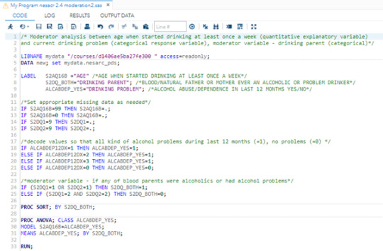
Without consideration of parents drinking history results had been the following:

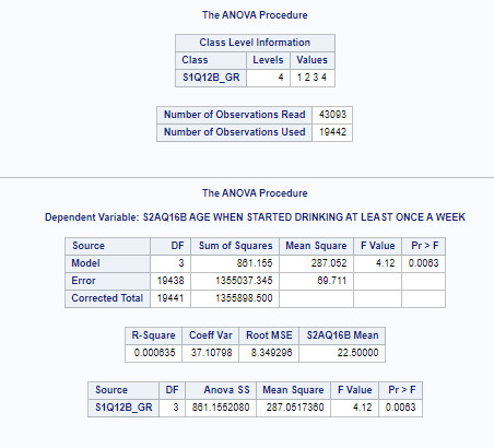
With p value <.0001 we can accept that age when person started drinking is significantly associated with him/her having alcohol dependency currently (0 - has no drinking problem, 1 - has alcohol dependency).

When moderator variable “having a drinking parent” is included in analysis, we can see this dependency even more clearly. p value in both cases remains <.0001.

When person had no drinking parent (=0), those who currently have alcohol dependency started drinking at later age (mean 20.60) than in analysis where parents history wasn’t considered.

When person had drinking parent (=1), those who have alcohol dependency started drinking at even younger age (mean 20.36) than in analysis where parents history wasn’t considered.

Please review my work. Thank you,

Edita

[editukas-blog1]

Generating a Correlation Coefficient, 3rd week assignment

Dear colleagues students,

for Pearson's correlation coefficient research I took possible association between 2 quantitative variables: age when person started drinking at least once a week and largest number of alcoholic drinks person consumes during period of heaviest drinking.

Here is program code:

To ensure whether variables have linear dependence, I draw scatter plot. Looks like there is negative correlation between variables.

Correlation procedure shows again negative correlation r=-0.26281 with p<0.0001 which shows significant association between these variables and lets us safely reject 0 hypothesis (which was that these variables are not associated).

Please review my work.

Thank you!

Edita

[editukas-blog1]

Chi Square Test of Independence, 2nd week assignment

Dear colleagues students,

Chi Square test of independence shows that household income in past 12 months (collapsed into 4 groups) and population alcohol abuse/dependence in last 12 months were significantly associated, X2 =57.249, 3 df, p<.0001.

As p is less than 0,00833 (0,05/6 as it is 6 comparisons), we can refuse 0 hypothesis that income groups and alcohol dependence are not related.

Post hoc comparisons by pairs shows that higher rates of alcohol abuse were seen in group with lowest income, “< $19,999″ when compared to any other income group (example below).

However, all other income groups: “< $34,999″, “< $59,999″ and “> 60,000″ when compared to each other in pairs have statistically very similar alcohol abuse levels (example below).

Please review my attempt on chi2 test.

Thank you in advance,

Edita

[editukas-blog1]

Analysis of Variance, 1st week assignment

Dear colleagues students,

here is my ANOVA analysis. As in my original research both variables are categorical, for this particular one I chose different research. From Nesacr Codebook I chose to check dependency between household income in last 12 months (categorical explanatory variable) and age when people started drinking at least once a week (quantitative response variable).

Null hypothesis - there is no difference in age when people started drinking at least once a week between people coming from household groups with different income in last 12 months. Alternative hypothesis is that there is difference.

Code:

Results:

We can see that household income and age when started drinking at least once a week are significantly associated. Mean is 22.5, F value 4.12 and p<0.01.

Post hoc comparisons of mean number of age when started drinking weekly show that people coming from households group 1 with yearly income up to $19,999 started drinking weekly significantly later (22,7664 y) than people coming from households group 4 with yearly income over $60,000 (22,2076 y). Another significant difference in drinking age is between income groups 3 (22.5824 y) and 4 (22,2076 y). All other comparisons were statistically similar.

Please review my work.

Kind Regards,

Edita

[editukas-blog1]

Visualizing Data, 4th week assignment

Dear colleagues students,

here is my last assignment of this course. We were asked to display data graphically.

My both variables ANXDEPTR and ALCABDEP_YES are categorical with only 2 categories in each (representing ’yes’ or ‘no’), so there is not much point in examining graphs center and spread. All of the following graphs are unimodal.

Here is program code.

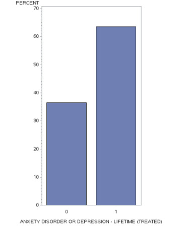
Observing univariate graph for first variable, “Anxiety disorder or depression - lifetime (treated)” we can see that in almost 65% of cases these diagnoses were treated (=1) and in 35% cases not treated (=0).

Observing univariate graph for second variable, “Alcohol abuse/dependence in last 12 months yes/no” we can see that more than 90% respondents reported that they have no alcohol problems (=0) and around 10% reported some kind of alcohol related problem (=1).

Observing bivariate graph we can see that people which were previously treated from anxiety/depression (=1)  experience alcohol problems in around 11% cases and those who were not treated (=0)  experience alcohol problems more often, in around 14% cases.

These results support my hypothesis that anxiety/depression treatment helps to resist alcohol abuse or dependence.

Hope you were convinced by my data research. Please leave comments if you wish.

Sincerely,

Edita

[editukas-blog1]

Data Management Decisions, 3rd week assignment

Dear colleagues students,

after this week lecture I re-wrote my program to use new possibilities.

I created 5 new variables in total which allowed me to achieve my data analysis goal easier. 

Below are results of this program. Last 2 frequencies provide me with required data.

ANXDEPRTR - I have counted population who have been diagnosed with general anxiety and/or depression and have been previously treated (=1) from these disorders or not treated (=0).

ALC_PROB - I counted if population corresponding variable ANXDEPRTR had recent (in last 12 months) problems with alcohol. ALC_PROB =0 means cases that haven’t been previously treated and have alcohol problems, ALC_PROB =1 means cases that have been previously treated and have alcohol problems.

This data allows me to check my hypothesis, if treatment from anxiety and/or depression helps to control alcohol abuse. According to results, 11% of population have been previously treated have alcohol problems and 14% of population  that have NOT been previously treated have such problems.

Please review my work, your comments are welcome.

Kind Regards,

Edita

[editukas-blog1]

SAS program, 2nd week assignment

Dear colleagues students,

let me show you my SAS code and it’s results for Nesarc data analysis. Sorry for extensive commenting, but I think it’s easier to understand.

And results:

My goal was to check how many of population, diagnosed with depression or general anxiety suffer from alcohol problems (in last 12 months) and if prior treatment of depression/anxiety has influence on alcohol abuse levels.

Possible values of ALCABDEP12DX are:

0. No alcohol diagnosis 1. Alcohol abuse only 2. Alcohol dependence only 3. Alcohol abuse and dependence

As you can see, alcohol problems among previously treated population (left side results) are slightly less common than among untreated (right side results), 88,65% vs 85,94% population with no alcohol diagnosis. It supports my hypothesis that anxiety/depression treatment helps to resist other dependencies.

Please comment on my work.

Thank you in advance,

Edita