joshuang307-blog - Tumblr blog

[joshuang307-blog]

Week 10- June 4th/6th

Presentations/wrapping up

Pictured here is my favorite slide from all of the presentations. I think that it’s pretty funny that the car-related project won the student contest both times, and that’s where this slide is from. 

Some cool things that I produced as a result of this presentation would be a cool Photoshop graphic to better illustrate what is happening (not to scale) and learning to edit and work with GIFs. 

a) If you were to pick one thing that you feel like you understand pretty well about aerodynamics now that you didn't at the start of 307, what is it and why?

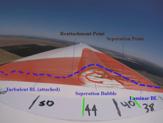
Separation bubbles on wings. I had always seen images in textbooks, but there is something about actually seeing it on a real plane in tangible oil visualization that makes me get it. Something else that I think i learned a lot about was using the wind tunnel to get useful numbers, and to run through things quickly while testing, instead of being confused or slow in the lab. 

b) If you were to pick one thing about aerodynamics that still confuses you, what is it and why?

Getting from x-y-z data to a proper Cp plot. I never really got the panel code to work properly, and I think that it was just a loose approximation of the real answer. I think that if you posted some kind of solution or talked in class explicitly about how those things are related, it would have helped me a lot.

c) What was your 307 highlight?

Miniprojects was fun and I think I learned the most doing it.

d) What was your 307 lowlight?

Messing around with those messy Excel files for the 4412 lab. I ended up getting it to work, but the 90 minutes I spent figuring it out could have been used to learn about aerodynamics.

e) For many of you, this'll be the last time you really engage with aerodynamics, since you prefer structures or controls or design or just anything else... for others, this course will have been a springboard to many future aerodynamic adventures. What do you think the future holds for you in aerospace engineering?

I think that I’m leaning towards structures/aerodynamics. I enjoyed the wind tunnel testing aspect of this class.

[joshuang307-blog]

6T Week 9- May 28th/May 30th + June 2nd

This week was spent wrapping up our mini-project presentation in terms of analysis and content on Monday/Wednesday, and then Saturday for an additional day of testing. On Monday we spent a lot of time analyzing the Go-Pro footage from the first round of testing and compiling data. I experimented with GIF making, our main form of visual data that we were going to utilize in our presentation. We agreed that because the testing was so inconclusive, we were going to do another test on a paved runway next Saturday. In our GoPro footage as well as additional pictures from the test site, we could clearly see the lack of separation of oil on the wing. We reconfirmed that our test procedure and materials were correct with one of Neiman’s associates who had done tests similar like this before. Therefore, we agreed that the dust particles that were caused by the dry dirt runway was the cause of our faulty oil flow. One regrettable thing for our test on Monday was that the GoPro did not capture the closest row, the one closest to the fuselage, arguably where the majority of the action occurred. We were only able to capture the tufting of the first 25% of chord for the first row, and judging from this row and the second row, the oscillations were only a few cm in magnitude, with no clear stalling characteristics. I think that if we were to do a test again, we would probably not get  anything meaningful, but I think it would be worth doing a higher resolution tuft grid that focused only on the wing only 0-5 inches from the fuselage, in contrast to our relatively large grid that extended up to 20 inches with a resolution of 3x3 inches. We concluded that there was no significant separation zone created by body, so that fairing the fuselage-wing junction would be somewhat beneficial, and would require significant design effort. We ended up thinking that it wasn’t worth the effort for the second test on Sat, and focused on getting that good oil data. 

On Saturday at the paved runway, there was no ridiculously thick cloud of dust generated on the paved runway, and so we were able to obtain laminar flow for the first 40% of chord, and obtained good oil pooling, as seen in the picture above. Since the pool location coincided with our predicted XFLR results, we agreed that it was only necessary to do one run. (fuel is expensive!)

The rest of the time in class was spent on doing research and learning about past tests on separation bubbles, data comparison, and results analysis of the videos. Some notable characteristics for the oil were that it appeared to settle into the pools within 5 minutes after takeoff, and the remaining 15 minutes only saw some of the pool fluid leaving the bubble due to small gusts and whatnot. Even with all the minor disturbances, the final oil bubble location chordwise did not change significantly. I do think that it would be interesting to find a way to make the oil slightly more viscous, so that we wouldn’t get any “bubble leakage”, as minor as it was anyways. 

In terms of why we think there is a separation bubble to begin with, it is important to keep in mind that the wing design is from the 60′s, and the engineers of that time had significantly less access to simulations and data analysis. That being said, I think that design renovations would be needed in order to truly eliminate the drag issues, but the turbulator solution proposed would still find its use with this type of glider aircraft/RC aircraft that operate at lower Reynolds numbers. Ideally, the airfoil would be designed and operated at the correct speeds, and so seeing separation bubbles on modern gliders would be in more niche situations. 

[joshuang307-blog]

Week 8- May 21st/May 23rd and May 26th(Saturday)

On May 21st and May 23rd, we refined our test plan, allocated test jobs, and developed our flow viz fluid. On May 21st we focused most of our efforts on creating and testing the fluid mixture. Initially, we followed the Delicious Paint recipe on Polylearn, which consisted of white pigment and motor oil. Dr Doig suggested that we add food dye in order to increase the visibility on the wing and also to test for viscosity and to see if we could get a desirable result by holding a painted wing behind the wind tunnel, as seen in the last photo. There were a lot of problems that we ran into for the fluid. The pigment was fairly grainy and did not dissolve into the oil base. It was still just pigment particles suspended in a clear oil, even after rigorous stirring for over ten minutes. When we tested the fluid in the wind tunnel, we found that either the fluid was too viscous and nothing happened, the fluid was too thin and nothing was observable, or even when the fluid was of proper viscosity, the oil would separate and leave behind an indiscernible trail of pigments. The addition of food coloring did not help either. The food coloring was water-based, and so when mixed into oil it would form into small droplets. It did not improve visibility at all. Overall, our testing with the fluid recipe was inconclusive. After looking around online we decided that we needed some kind of oil-based coloring. The viscosity of the motor oil was good enough, but it was still very hard to see any changes even after moving air over the wing for at least 10 minutes. 

Neiman reached out to one of his glider friends who had successfully completed this sort of flow viz test before, and he recommended us to use old motor oil. Unfortunately, we were not able to get our hands on any of the stuff until Saturday, and so we did not get to test it in the wind tunnel before the actual test. 

On May 27th, we went out to Avenal Airport to do our testing. Flying conditions were pretty good. The test pilot noted that there was a lot of active air, but there were few clouds and was pretty early in the morning. 

Unfortunately, the oil separation patterns were not as clear as we had hoped. You can see a faint line in the oil patterns at around the ~45% chord mark, but it not conclusive. In addition to the oil we also tufted the wing section close to the wing roots. We were able to successfully mount two Go-Pros on the wing to monitor both the oil and the tufts. We did the velocity trials at both 50 and 60 knots. After the second test we decided as a group that it was unnecessary to do the 70 knot trial; there was no observable difference between the 50 and 60, and because the main goal of the variable speeds was for repeatability, and because each trial was fairly expensive, we decided to leave it at the two runs. We attributed the lack of significant oil pattern formation in that there was never really a transition from laminar to turbulent, since we found that because the runway was dirt and because it was dry, the tow plane kicked up a massive cloud of dust upon each take off. A lot of dust particles would stick onto the oil in the beginning of each trial, and so we speculated that the dust particles that were adhered to the leading edge would cause all the downstream flow to be turbulent. The tests that his friend had recommended were done on a paved road. In this way we concluded that the lack of desired results was not due to the fluid paint viscosity or material, but the testing location and conditions. 

[joshuang307-blog]

Week 7- May 14th/May 16th

On May 14th, our group did the force balance lab. It was the classic bread-and-butter test that we were supposed to do in 303. Now that we have a new load cell, we could get around to it! Last week, we had developed a code to read in and to create basic plots given the Excel formatted force balance data. In lab, were were testing two finite 4412 wings. We kept the Reynolds number constant between the two wings and then ran them in the tunnel at varying angles of attack. In order to match the Reynolds numbers we had two different wind tunnel speeds. Some minor issues that our group ran into when testing was that we missed taking wind off data for one of our sets. We were able to figure it out and just took additional data after our set without zeroing to obtain values that we could subtract later on. These values would be those caused by the obstructions of the plates that were part of the sting mount. Some things that we pondered as we ran the lab: Given the same Reynolds number, would the high aspect or the low aspect wing result in a better L/D and other aerodynamic characteristics, and why?  I think that the high aspect ratio will have better results, because though both wings will experience vortex drag, the strength of the vortex may also vary, because the size of the wingtip is larger for the lower aspect ratio. However, I must consider that  the low aspect ratio wing will have less surface area that will be influenced by the created vortices.  Typically, this is the reason that very high aspect ratio wings, such as those found on gliders, have less induced drag.

Some potential problems that we may run into as we go more in-depth with the analysis would be potential sources of error, and how we may relate them to our trends. Based on our uncorrected, immediate plots during the testing session, our values for CL seem to be slightly under the values provided from airfoil tools at the relevant Reynolds numbers.

On May 16th, we broke up into our mini-projects. I was grouped up with Neiman Walker and Robseth Taas. We spent the day in the library doing research and formulating a test plan. We plan to test next Saturday at the gliderport at Avenal. Essentially, our main test goal was to be able to define the chordwise location of the laminar separation bubble of a Glasflugel H-201 glider. Ideally, within given time and financial constraints, we want to be able to fit turbulators along the wingspan to mitigate the negative effects of the laminar separation bubbles. Additionally, we will monitor the effects of induced body drag near the wing roots. We plan to capture these characteristics with the use of flow viz fluid, and tufting, captured during the flight with Go-Pros. 

In the last picture you can see our process through choosing our velocity based on the polar plot for our glider, in the 50-80 knot range. On our final test plan, we chose the velocities of 50,60,and 70 knots. Some additional considerations that we had were price per flight (over 30 dollars in fuel for the tow plane)

[joshuang307-blog]

Week 6- May 7th/May 9th

 On May 7th, we gave our presentation on the flow viz project. While we were presenting, I noticed that we had prepared too much information and had not distilled it down. It ended up going too long but I think that we were able to successfully introduce and describe what we had accomplished. I think that I could have played a greater part in shortening everyone else’s slides, not just my own, and could have probably rewritten what I had originally planned to say.

Code planned for the testing of the wing section. Apparently we get to do the classic wind tunnel test (again?) but with a real load cell this time. During May 9th I spent the whole class period working on code for this lab. There were a lot of issues that had to do almost entirely with the formatting of the sample data that we were given. The most irritating thing was that the files were xls files, but xlsread had a hard time with them so I had to manually rename each file to a .xlsx. Most of the others in my lab section also had a lot of problems with reading the data into Matlab... Additionally, each Excel file had 3 useful sheets of information on them. In the end, I abandoned hard coding each file in and used a “dir” command to make one giant matrix with all of the data for the x, y, and z components. The main goal here was to be able to successfully read in the excel files, and to be able to group and access individual numbers properly. I wrote up a quick plot for Cl that at least has the right slope to it. The main issue here was that using the “dir” command created an order for angles of attack of 0,10,15, and 5. Because these angles were out of order, I had to manually reassign the angles and their force pairs. This will probably be very annoying when we take our data for real and have many more angle of attack measurements. In this case, I think that I will replace the TA’s naming system for something that is more friendly to the “sort by alphabet” naming system that “dir” uses. Something that I am not sure for calculating the lift forces is what each data set is for. To my understanding, Wing ON and Wing OFF are separate things that we are looking for, and so in order to get the proper force values, we simply subtract the corresponding Wind OFF value from the sets? Or is it (Wing ON- Wing OFF - Wind OFF) that gives us the true force values? Additionally, in the lab manual it says that y is drag and z is negative lift (the wing is upsidedown), so then where do the x values go? It makes sense that most of the x values in the provided data set are approximately zero, so if it turns out that these values are all insignificant, then I think that not including them in the calculations would maybe be a good idea. Right now, I think that I could get visual plots for CL and CD pretty easily, the only problem is figuring out where the wing off/wind off data factors into the main calculations. 

[joshuang307-blog]

Week 5- April 30th/May 2nd 

This week was flow-viz testing! At the start of week 5, our group had already completed the bridge model and we were ready to start planning our experiment in earnest. Our main goals were to be able to use slow motion video to capture the oscillatory behaviors of the bridge. Specifically, we wanted to find the frequencies of the shedding vortex, the cables, and the torsional deck oscillations. On Monday we started to think of a test plan and tried to plan out some considerations. Honestly, we had no real idea of what kinds of numbers to expect, so we went into the test not knowing exactly what kind of behaviors we could expect, and not knowing the speeds that we could run at. My main concern was that the bridge would simply be too strong or too weak, and so we tried to account for this by making the deck section super flimsy yet modifiable. We planned to slowly increase the speed of the wind tunnel, and make adjustments with tape based on the results.

We quickly found that because our deck was made entirely out of light cardboard and that it was held in place only by the suspension of the cables, wind tunnel velocities above 10 m/s caused the deck to flip over. This was actually expected because when we were carrying the bridge model to the lab, a gust of wind actually blew the deck over (Picture 2). This is a super interesting phenomenon because it also suggests that our deck provides lift, or perhaps the strings are the moment arm that gets moved by the incoming flow... This was not a hard fix, we decided to use aluminum tape to tape down the ends of the bridge to stop it from flipping over. This fixed the issue, but it created many more. I was not sure how we could properly record and account for the increase in the effective load on the bridge caused by the tension of the tape. This increased the curvature of the deck and the tension in each cable. Additionally, it was hard to tell if the tape was applied the same way to both ends. Thinking about the overall effect, I think that for the purpose of determining frequency, the tape would not have made a significant difference for the torsional and shedding frequency, but I feel that the oscillation of the cables was greatly influenced by the tape. In our earliest videos, before we taped the deck down, the cables got blown at nearly 30 degrees away from the vertical, and looked super loose. This is definitely something worth investigating.

In the first picture you can see how we taped down the deck, and note the extent to which the cables have been displaced. I think that to do a better version of this test we would need more knowledge on bridge mechanics and better designs and materials for the bridge. 

[joshuang307-blog]

Week 4 - April 23rd/April 25th

[joshuang307-blog]

Week 3 - April 16th/April 18th

This week was wake survey testing week. Our lab group met up in the wind tunnel and after a brief discussion of the test plan we started to get underway. It is important to note that the LabVue setup was changed, with the addition of the wake pressure measurements, freestream measurements, which occupied the port slots 1-4, which would mean small changes to our matlab code. Our group decided on measuring the wake at the angles of attack of 3,-3, and 6. We would visually line up the tailing edge to the 3D traverse, to which a pressure sensor was mounted. These values for y-traverse displacement in millimeters were displayed on the orange board as pictured. For this testing period, I was making small 2-4 millimeter displacements for the traverse and monitoring the progress of the the pressure sensors. In particular, I was making the comparison between the freestream pressure and the wake pressure. The pressure deficit that occured behind the trailing edge would be larger the closer it was to the probe. My main job was to make sure to incrementally change the displacement depending on how large the changes in pressure were for Port 4, the wake probe, as well as compare to the freestream pressure. If there was too minute of a change, after the new conditions settled, I would not record any data and instead make another change in the traverse displacement.  When the wake pressure was within ~2 of the freestream pressure, I would know that the probe had moved enough far away to complete the data set. Something strange that I noticed initially when comparing values to the previous test were the disparity in numbers for pressure. 

[joshuang307-blog]

Week 2 - April 9th (Monday)

This week our group finally had our allotted time in the wind tunnel! The first ninety minutes of class was spent in the conference room as we worked on finalizing our test plan and working on panel code. For our first run we planned to run the wind tunnel at 10 m/s and start from a negative angle of attack, increase it to past stall, then decrease the angle of attack until reattachment. Our main testing goals were to find the zero angle of attack, the stall angle, and the reattachment angle. Typically we know that the reattachment angle ends up being lower than the stall angle, and so we planned for this with our angle distribution. Our intended angles for testing were: -5, -4, -3, 0, 3, 6, 9, 10, 11, 12, 13, 14, 15, 16, 17, 18, 15, 12, 11, 10, 9. We would run through this set of angles twice, once at 10m/s and once at 15 m/s. 

When it was finally our time to test, the whole group walked over, only to find that the group before us was running late. So we spent maybe ten minutes waiting outside.  Once we got into the lab, Doig explained the basic roles and how things would run. One notable contribution Doig made was to recommend us to run the tunnel at 25 m/s instead of 15 m/s, as the Reynolds number would become much higher in the turbulent case. We had originally planned to keep it at laminar, but we agreed that we would probably see more of a change with this higher speed. 

While we were in the setup phase I came up with an efficient naming scheme, where the three things that were changing were run, velocity, and angle of attack. Therefore our matlab  syntax could be r_v_a_.mat. I had pictured the runs being run 1 for our first set of data and run 2 for our second set of data. When I proposed this, Josh B improved upon it by saying that for every angle that we took, we would change the run number by one. This meant that every single data set that we took would have a different run number, and that all of our data would be ordered chronologically in the order that we took them in. This was a great idea. This would also help differentiate the repeated angles as we went up and then back down. Also, for negative angles of attack, ‘n’ would represent the negative sign. Our very first run would therefore by “r1v1an5.mat’. 

For roles, we decided to switch roles just two times, in order to give us more time to test efficiently (as we were running late from the group before us). We had 42 planned data samples! I chose to start at the angle winch. We agreed to use hand signals to show the current angle of attack, followed by a thumbs up by both the winch operator and someone in the control room. I quickly setup a basic table for all the angle attachments and a column next to it for notes on whatever happened in the test section, and a column to put a check mark in order to keep track of which ones had been completed. My accuracy I would estimate at around +/- .25 deg.

Everything ended up running very smoothly and we were all pretty organized. For the first half of the lab, Josh B was on LabVUE, Josh D was communicating with me and changing what was on the whiteboard and doing RPM changes, and Noah was checking all of the data on matlab through our script, and I was changing the angle of attack and taking observational notes. We had a change to our angle matrix as we found that we had an earlier reattachment, and so we added angle 14 and eliminated 12,11,10 and 9 as we decided those were no longer needed. Most of the experimental notes had to do with what the tuft was doing, such as oscillations and directions (which changed when stall occurred). We had stall at 16 degrees for 15 m/s and at 13 degrees for 25 m/s. The tuft would oscillate rapidly and then switch directions from pointing towards to trailing edge and then once in full stall, towards the leading edge.

Week 2 - April 11th (Wednesday)

Our group all met up in the conference room again and went to work with completing and ironing out the panel code, setting up the lab memo format, and looking at our data sets that we collected on monday.

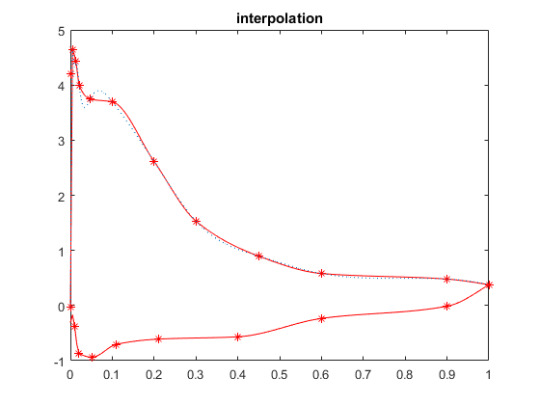
While Josh B and Noah worked on the panel code, I worked on trying to interpolate and fit a curve to our data points. I separated the ports into top and bottom, so that I could generate separate lines for both the top and the bottom.  Looking at the posted interpolation plot for r32v2a16 my curve looks very good, but there appears to be very minor vertical offset. I don’t know if this is because I’m not accounting for something. It seems pretty consistent with the panel code plots, however. Later, Josh D and I started to iron out the Tech memo. Since some of our plots still did not make any sense, we focused on everything except for analysis. Generally speaking, our data for v=25 m/s looked very good, but some of the 10m/s plots had funny shapes for cp and then for l/d.

[joshuang307-blog]

Week 1 - April 2nd (Monday)

We were given some sample data for the infinite NACA 4412 wing measured at a wind tunnel velocity of 10m/s and an angle of attack of 10 degrees. Since I had already created a panel code for a 2d NACA 4412 airfoil in AERO306, I only had to change a few things to create a x/c vs cp plot. I also worked on the test plan and calculated Reynolds values for testing, as well as the prospective velocities. As a group we agreed to later do a tunnel RPM to velocity conversion after we took our data on the following Monday.

Week 1 - April 4th (Wednesday) 

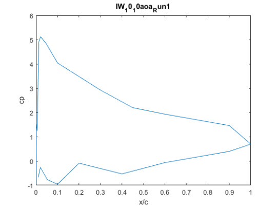
After finishing the test plan, I decided to make my own code reader. I think that it would be relatively painless if we copied our TA Tynan’s filename structure, since it works pretty good. He uses  IW_10_10aoa_Run1. This leaves 3 changing variables: the velocity, aoa, and run number. In matlab this is just 3 loops.

I created a small code to read in the given data from the TA and converted the raw pressure readings into average cp values per port number, and then created an x/c vector using the information that was given for the location of the ports. Using this I was able to create a basic x/c vs cp plot. I had to hard code in ports 8 and 16 because the data points were extremely off, but this could be due to poor data. I decided not to do much more hard coding until we get our actual data points later. 

Doing a quick comparison between the plots of the data vs the panel code, I can see that the general shape of the curves is consistent, though a lot of fine tuning will be needed to eliminate the points that don’t make sense, especially for the negative cp values.