kushaldube - Tumblr blog

kushaldube · 4 years ago

Text

Data Management and Visualization - Week 3

Hello, I am Kushal Dube. This Blog is a part of the Data Management and Visualization course by Wesleyan University via Coursera. The assignments in this course are to be submitted in the form of blogs and hence I chose Tumblr as suggested in the course for submitting my assignments. You can read the week 1 blog using these links: Week-1, Week-2.

Here is my codebook:

Research Question:

Is there any relation between life expectancy and alcohol consumption? Is there any relation between Income and alcohol consumption?

Assignment 3:

This assignment contains data management for respective topics. We have to make and implement decisions about data management for the variables. Data Management is a process to store, organize, and maintain data. Security of data is very important to secure the data which is a part of Data Management.

Blog contains:

- Removing missing data rows - Make a group of income, alcohol consumption, and life expectancy - Show frequency distribution before and after grouping

Data Dictionary:

Code:

Step 1: Importing Libraries

#import the libraries import pandas import numpy from collections import OrderedDict

Step 2: Read the specific columns of the dataset and rename the columns

data=pandas.read_csv('gapminder.csv',low_memory=False, skip_blank_lines=True, usecols=['country','incomeperperson','alcconsumption','lifeexpectancy']) data.columns=['country','income','alcohol','life'] ''' #Variable Descriptions alcohol="2008 alcohol consumption per adult (liters,age 15+)" income="2010 Gross Domistic Product per capita in constant 2000 US$" life="2011 life expectancy at birth (years)" ''' data.info()

Output:

<class 'pandas.core.frame.DataFrame'> RangeIndex: 213 entries, 0 to 212 Data columns (total 4 columns): # Column Non-Null Count Dtype --- ------ -------------- ----- 0 country 213 non-null object 1 income 213 non-null object 2 alcohol 213 non-null object 3 life 213 non-null object dtypes: object(4) memory usage: 6.8+ KB

Step 3: convert arguments to a numeric types from .csv files

for dt in ('income','alcohol','life'): data[dt]=pandas.to_numeric(data[dt],errors='coerce') data.info()

Output:

<class 'pandas.core.frame.DataFrame'> RangeIndex: 213 entries, 0 to 212 Data columns (total 4 columns): # Column Non-Null Count Dtype --- ------ -------------- ----- 0 country 213 non-null object 1 income 190 non-null float64 2 alcohol 187 non-null float64 3 life 191 non-null float64 dtypes: float64(3), object(1) memory usage: 6.8+ KB

Step 4: Drop the missing data rows

data=data.dropna(axis=0,how='any') print(data.info())

Output:

<class 'pandas.core.frame.DataFrame'> Int64Index: 171 entries, 1 to 212 Data columns (total 4 columns): # Column Non-Null Count Dtype --- ------ -------------- ----- 0 country 171 non-null object 1 income 171 non-null float64 2 alcohol 171 non-null float64 3 life 171 non-null float64 dtypes: float64(3), object(1) memory usage: 6.7+ KB None

Step 5: Display absolute and relative frequency

c2=data['income'].value_counts(sort=False) p2=data['income'].value_counts(sort=False,normalize=True) c3=data['alcohol'].value_counts(sort=False) p3=data['alcohol'].value_counts(sort=False,normalize=True) c4=data['life'].value_counts(sort=False) p4=data['life'].value_counts(sort=False,normalize=True) print("***************************************************") print("****************Absolute Frequency****************") print("Income Per Person: ") print("Income Freq") print(c2) print("Alcohol Consumption: ") print("Income Freq") print(c3) print("Life Expectancy:") print("Income Freq") print(c4) print("***************************************************") print("****************Relative Frequency****************") print("Income Per Person: ") print("Income Freq") print(c2) print("Alcohol Consumption: ") print("Income Freq") print(c3) print("Life Expectancy:") print("Income Freq") print(c4)

Output:

*************************************************** ****************Absolute Frequency**************** Income Per Person: Income Freq 1914.996551 1 2231.993335 1 1381.004268 1 10749.419238 1 1326.741757 1 .. 5528.363114 1 722.807559 1 610.357367 1 432.226337 1 320.771890 1 Name: income, Length: 171, dtype: int64 Alcohol Consumption: Income Freq 7.29 1 0.69 1 5.57 1 9.35 1 13.66 1 .. 7.60 1 3.91 1 0.20 1 3.56 1 4.96 1 Name: alcohol, Length: 165, dtype: int64 Life Expectancy: Income Freq 76.918 1 73.131 1 51.093 1 75.901 1 74.241 1 .. 74.402 1 75.181 1 65.493 1 49.025 1 51.384 1 Name: life, Length: 169, dtype: int64 *************************************************** ****************Relative Frequency**************** Income Per Person: Income Freq 1914.996551 1 2231.993335 1 1381.004268 1 10749.419238 1 1326.741757 1 .. 5528.363114 1 722.807559 1 610.357367 1 432.226337 1 320.771890 1 Name: income, Length: 171, dtype: int64 Alcohol Consumption: Income Freq 7.29 1 0.69 1 5.57 1 9.35 1 13.66 1 .. 7.60 1 3.91 1 0.20 1 3.56 1 4.96 1 Name: alcohol, Length: 165, dtype: int64 Life Expectancy: Income Freq 76.918 1 73.131 1 51.093 1 75.901 1 74.241 1 .. 74.402 1 75.181 1 65.493 1 49.025 1 51.384 1 Name: life, Length: 169, dtype: int64

Step 6: Make groups in variables to understand such research question

minMax=OrderedDict()

dict1=OreredDict()

dict1['min']=data.life.min()

dict1['max']=data.life.max()

minMax['life']=dict1

dict2=OreredDict()

dict2['min']=data.life.min()

dict2['max']=data.life.max()

minMax['income']=dict2

dict3=OreredDict()

dict3['min']=data.life.min()

dict3['max']=data.life.max()

minMax['alcohol']=dict3

#df=pandas.DataFrame([minMax['income'],minMax['life'],minMax['alcohol'],index=['income','life','alcohol']])

df = pandas.DataFrame([minMax['income'],minMax['life'],minMax['alcohol']], index = ['Income','Life','Alcohol'])

print(df.sort_index(axis=1,ascending=False))

dummyData=data.copy()

#Maps

income_map={1: '>=100 <5k', 2: '>=5k <10k', 3: '>=10k <20k', 4: '>=20K <30K', 5: '>=30K <40K', 6: '>=40K <50K' }

life_map={1: '>=40 <50', 2: '>=50 <60', 3: '>=60 <70', 4: '>=70 <80', 5: '>=80 <90'}

alcohol_map={1: '>=0.5 <5', 2: '>=5 <10', 3: '>=10 <15', 4: '>=15 <20', 5: '>=20 <25'}

dummyData['income'] = pandas.cut(data.income,[100,5000,10000,20000,30000,40000,50000], labels=['1','2','3','4','5','6'])

print(dummyData.head(10))

dummyData['life'] = pandas.cut(data.life,[40,50,60,70,80,90], labels=['1','2','3','4','5'])

print(dummyData.head(10)

#dummyData['alcohol'] = pandas.cut(data.alcohol,[0.5,5,10,15,20,25], labels=['1','2','3','4','5'])

dummyData['alcohol'] = pandas.cut(data.alcohol,[0.5,5,10,15,20,25], labels=['1','2','3','4','5'])

print(dummyData.head(10)

Output:

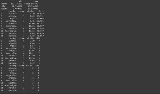
Step 7: Frequency Distribution of new grouped data

Full Code:

#Import the libraries

import pandas

import numpy

from collections import OrderedDict

#from tabulate import tabulate, tabulate_formats

data = pandas.read_csv('gapminder.csv', low_memory=False, skip_blank_lines=True, usecols=['country','incomeperperson', 'alcconsumption', 'lifeexpectancy'])

data.columns=['country', 'income', 'alcohol', 'life']

'''

# Variables Descriptions

alcohol = “2008 alcohol consumption per adult (liters, age 15+)”

income = “2010 Gross Domestic Product per capita in constant 2000 US$”

life = “2011 life expectancy at birth (years)”'''

data.info()

for dt in ('income','alcohol','life') :

data[dt] = pandas.to_numeric(data[dt], errors='coerce')

data.info()

nullLabels =data[data.country.isnull() | data.income.isnull() | data.alcohol.isnull() | data.life.isnull()]

print(nullLabels)

data = data.dropna(axis=0, how='any')

print (data.info())

c2 = data['income'].value_counts(sort=False)

p2 = data['income'].value_counts(sort=False, normalize=True)

c3 = data['alcohol'].value_counts(sort=False)

p3 = data['alcohol'].value_counts(sort=False, normalize=True)

c4 = data['life'].value_counts(sort=False)

p4 = data['life'].value_counts(sort=False, normalize=True)

print("***************************************************")

print("****************Absolute Frequency****************")

print("Income Per Person: ")

print("Income Freq")

print(c2)

print("Alcohol Consumption: ")

print("Income Freq")

print(c3)

print("Life Expectancy:")

print("Income Freq")

print(c4)

print("***************************************************")

print("****************Relative Frequency****************")

print("Income Per Person: ")

print("Income Freq")

print(c2)

print("Alcohol Consumption: ")

print("Income Freq")

print(c3)

print("Life Expectancy:")

print("Income Freq")

print(c4)

minMax = OrderedDict()

dict1 = OrderedDict()

dict1['min'] = data.life.min()

dict1['max'] = data.life.max()

minMax['life'] = dict1

dict2 = OrderedDict()

dict2['min'] = data.income.min()

dict2['max'] = data.income.max()

minMax['income'] = dict2

dict3 = OrderedDict()

dict3['min'] = data.alcohol.min()

dict3['max'] = data.alcohol.max()

minMax['alcohol'] = dict3

df = pandas.DataFrame([minMax['income'],minMax['life'],minMax['alcohol']], index = ['Income','Life','Alcohol'])

print (df.sort_index(axis=1, ascending=False))

dummyData = data.copy()

# Maps

income_map = {1: '>=100 <5k', 2: '>=5k <10k', 3: '>=10k <20k',

4: '>=20K < 30K', 5: '>=30K <40K', 6: '>=40K <50K' }

life_map = {1: '>=40 <50', 2: '>=50 <60', 3: '>=60 <70', 4: '>=70 <80', 5: '>=80 <90'}

alcohol_map = {1: '>=0.5 <5', 2: '>=5 <10', 3: '>=10 <15', 4: '>=15 <20', 5: '>=20 <25'}

dummyData['income'] = pandas.cut(data.income,[100,5000,10000,20000,30000,40000,50000], labels=['1','2','3','4','5','6'])

print(dummyData.head(10))

dummyData['life'] = pandas.cut(data.life,[40,50,60,70,80,90], labels=['1’,’2','3','4','5'])

print(dummyData.head(10))

dummyData['alcohol'] = pandas.cut(data.alcohol,[0.5,5,10,15,20,25], labels=['1','2','3','4','5'])

print (dummyData.head(10))

c2 = dummyData['income'].value_counts(sort=False)

p2 = dummyData['income'].value_counts(sort=False, normalize=True)

c3 = dummyData['alcohol'].value_counts(sort=False)

p3 = dummyData['alcohol'].value_counts(sort=False, normalize=True)

c4 = dummyData['life'].value_counts(sort=False)

p4 = dummyData['life'].value_counts(sort=False, normalize=True)

print("***************************************************")

print("****************Absolute Frequency****************")

print("Income Per Person: ")

print("Income Freq")

print(c2)

print("Alcohol Consumption: ")

print("Income Freq")

print(c3)

print("Life Expectancy:")

print("Income Freq")

print(c4)

print("***************************************************")

print("****************Relative Frequency****************")

print("Income Per Person: ")

print("Income Freq")

print(c2)

print("Alcohol Consumption: ")

print("Income Freq")

print(c3)

print("Life Expectancy:")

print("Income Freq")

print(c4)

0 notes

kushaldube · 4 years ago

Text

Data Management and Visualization - Week 2

Assignment 2

In this assignment, we first had to choose the language which we will be using for coding for which I chose Python as it is an easy to learn and a very popular language with many features and advantages. Then we have to write code through which we can load the dataset in the memory and calculate the frequency distribution of chosen variables.

#importing the libraries import pandas import numpy from tabulate import tabulate #read data from .csv file data = pandas.read_csv('gapminder.csv', low_memory=False) print ('Number of observations: ',len(data)) #number of observations (rows) print ('Number of variables: ',len(data.columns)) # number of variables (columns) print('*\t*\t*\t*\t*\t*\t*\t*\t*\t*') print('\nCounts for Country - Data available for which country') c1=data['country'].value_counts(sort=False) #count of country print(c1) print('\nPercentages for Country') p1=data['country'].value_counts(sort=False, normalize=True) #percentage of country print(p1) print('*\t*\t*\t*\t*\t*\t*\t*\t*\t*') print('\nCounts for Income per person - Countrywise average income per person') c2=data['incomeperperson'].value_counts(sort=False) print(c2) print('\nPercentages for Income per person - Countrywise average income per person') p2=data['incomeperperson'].value_counts(sort=False, normalize=True) print(p2) print('*\t*\t*\t*\t*\t*\t*\t*\t*\t*') print('\nCounts for Alcohol comsumption - in litres') c3=data['alcconsumption'].value_counts(sort=False) print(c3) print('\nPercentages for Alcohol comsumption - in litres') p3=data['alcconsumption'].value_counts(sort=False, normalize=True) print(p3) print('*\t*\t*\t*\t*\t*\t*\t*\t*\t*') print('\nCounts for Life expentancy - in years') c4=data['lifeexpectancy'].value_counts(sort=False) print(c4) print('\nPercentages for Life expentancy - in years') p4=data['lifeexpectancy'].value_counts(sort=False, normalize=True) print(p4) missings=[['Var','Missings']] for var in ('incomeperperson','alcconsumption','lifeexpectancy'): missings.append([var,data[var].value_counts()[' ']]) print(tabulate(missings,headers="firstrow"))

Code Description:

Step 1: Import necessary libraries Step 2: Read a data file Step 3: Count the variable rows and display them along with the variable column

Output:

runfile('D:/Programming/Coursera/Data Management and Visualization/script.py', wdir='D:/Programming/Coursera/Data Management and Visualization') Number of observations: 213 Number of variables: 16 * * * * * * * * * * Counts for Country - Data available for which country Afghanistan 1 Albania 1 Algeria 1 Andorra 1 Angola 1 .. Vietnam 1 West Bank and Gaza 1 Yemen, Rep. 1 Zambia 1 Zimbabwe 1 Name: country, Length: 213, dtype: int64 Percentages for Country Afghanistan 0.004695 Albania 0.004695 Algeria 0.004695 Andorra 0.004695 Angola 0.004695 Vietnam 0.004695 West Bank and Gaza 0.004695 Yemen, Rep. 0.004695 Zambia 0.004695 Zimbabwe 0.004695 Name: country, Length: 213, dtype: float64 * * * * * * * * * * Counts for Income per person - Countrywise average income per person 23 1914.99655094922 1 2231.99333515006 1 21943.3398976022 1 1381.00426770244 1 .. 5528.36311387522 1 722.807558834445 1 610.3573673206 1 432.226336974583 1 320.771889948584 1 Name: incomeperperson, Length: 191, dtype: int64 Percentages for Income per person - Countrywise average income per person 0.107981 1914.99655094922 0.004695 2231.99333515006 0.004695 21943.3398976022 0.004695 1381.00426770244 0.004695 5528.36311387522 0.004695 722.807558834445 0.004695 610.3573673206 0.004695 432.226336974583 0.004695 320.771889948584 0.004695 Name: incomeperperson, Length: 191, dtype: float64 * * * * * * * * * * Counts for Alcohol comsumption - in litres .03 1 7.29 1 .69 1 10.17 1 5.57 1 .. 7.6 1 3.91 1 .2 1 3.56 1 4.96 1 Name: alcconsumption, Length: 181, dtype: int64 Percentages for Alcohol comsumption - in litres .03 0.004695 7.29 0.004695 .69 0.004695 10.17 0.004695 5.57 0.004695 7.6 0.004695 3.91 0.004695 .2 0.004695 3.56 0.004695 4.96 0.004695 Name: alcconsumption, Length: 181, dtype: float64 * * * * * * * * * * Counts for Life expentancy - in years 48.673 1 76.918 1 73.131 1 22 51.093 1 ... 75.181 1 72.832 1 65.493 1 49.025 1 51.384 1 Name: lifeexpectancy, Length: 190, dtype: int64 Percentages for Life expentancy - in years 48.673 0.004695 76.918 0.004695 73.131 0.004695 0.103286 51.093 0.004695 ... 75.181 0.004695 72.832 0.004695 65.493 0.004695 49.025 0.004695 51.384 0.004695 Name: lifeexpectancy, Length: 190, dtype: float64

Conclusion:

Here the variables are not categorical. That is the reason why the percentage is unusable.

2 notes · View notes

kushaldube · 4 years ago

Text

Data Management and Visualization - Week 1

Assignment 1

In this, we have to choose one of five codebooks provided in the course and a subcategory along with two topics/variables on which we want to research.

1. Choose a data set that you would like to work with

After reviewing all the codebooks provided, I decided to proceed with the portion of GapMinder data. This data includes one year of numerous country-level indicators of health, wealth, and development. My reason for choosing this was that it has data from all countries in multiple fields related to health, income, etc.

2. Identify a specific topic of interest

Alcohol consumption is injurious to health and life expectancy is affected due to it. With this, I want to investigate the correlation between the expectancy of life and alcohol consumption when I analyzed the GapMinder codebook.

3. Prepare a codebook of your own

Multiple variables were provided in the portion of GapMinder which is itself a little part of the proper documentation. Here I have mentioned only the variables that I think I will use, namely incomeperperson, alcconsumption and lifeexpectancy as variables

4. Identify a second topic that you would like to explore in terms of its association with your original topic

While looking at the codebook, I thought that there might be a possibility that the urban rate is connected to alcohol consumption. We can see in urban areas, people are less aware of their health and consume more toxic. Hence, the second topic which I would like to explore is urbanrate.

5. Add questions/items/variables documenting this second topic to your personal codebook

Is there any relation between alcohol consumption and the urban rate?

Is there any relation between life alcohol consumption and expectancy?

Is there any relation between alcohol consumption and Income?

Updated codebook:

6. Perform a literature review to see what research has been previously done on this topic

For the research of the topic I used google scholar as the go-to website, for the relation between urbanrate and alcohol consumption, research papers are not available for the topic. On searching about this on the google search engine I got to know that there is no direct relation between these two. The relation as in terms of stress and culture. Those can be in the city and urban are also. So I don’t have to consider this term(urbanrate). On the other hand for the relationship between life expectancy and alcohol consumption, many articles were present, this was the same for income and alcohol consumption. Some of the articles with their overview are as follows.

Lifetime income patterns and alcohol consumption: Investigating the association between long- and short-term income trajectories and drinking Overview: In this paper, the authors evaluated the relationship between long-term and short-term measures of income. They used the data of the US Panel Study on Income Dynamics. They also gave inferences like the low income associated with heavy consumption. “Lifetime income patterns may have an indirect association with alcohol use, mediated through current socioeconomic position.”

A Review of Expectancy Theory and Alcohol Consumption According to their study, “Expectancy manipulations and alcohol consumption: three studies in the laboratory have shown that increasing positive expectancies through word priming increases subsequent consumption and two studies have shown that increasing negative expectancies decreases it”.

Alcohol-related mortality by age and sex and its impact on life expectancy: Estimates based on the Finnish death register In this article, the author studied plausible results on the connection between alcohol-related mortality and age and sex. Here are few statistics, “According to the results, 6% of all deaths were alcohol-related. These deaths were responsible for a 2-year loss in life expectancy at age 15 years among men and 0.4 years among women, which explains at least one-fifth of the difference in life expectancies between the sexes. In the age group of 15–49 years, over 40% of all deaths among men and 15% among women were alcohol-related. In this age group, over 50% of the mortality difference between the sexes results from alcohol-related deaths”.

7. Based on your literature review, develop a hypothesis about what you believe the association might be between these topics. Be sure to integrate the specific variables you selected into the hypothesis.

After exploring such articles, they are enough to establish the correlation between alcohol consumption and life expectancy and also with Income (apart from these three). After certain observation, the following is my hypothesis:

Alcohol consumption is highly correlated with life expectancy.

The social culture, group of people associated with person, stress, and Income have a direct correlation with alcohol consumption.

Urban rate is not directly connected to alcohol consumption.

Final Codebook:

Reference:

Cerdá, Magdalena, et al. “Lifetime Income Patterns and Alcohol Consumption: Investigating the Association between Long- and Short-Term Income Trajectories and Drinking.” Social Science & Medicine, vol. 73, no. 8, 2011, pp. 1178–1185., doi:10.1016/j.socscimed.2011.07.025.

Jones, Barry T., et al. “A Review of Expectancy Theory and Alcohol Consumption.” Addiction, vol. 96, no. 1, 2001, pp. 57–72., doi:10.1046/j.1360–0443.2001.961575.x.

Makela, P. “Alcohol-Related Mortality by Age and Sex and Its Impact on Life Expectancy.” The European Journal of Public Health, vol. 8, no. 1, 1998, pp. 43–51., doi:10.1093/eurpub/8.1.43.

3 notes · View notes