learning2program

[learning2program]

Exploring the 3sum problem

Today, we’ll be exploring a bad solution to the 3sum problem.

First and foremost, I wrote this very late at night and so there are probably many typos. I’ve been meaning to work on some more stuff for this over the summer, but research and real life has eaten up a lot of my time. I’m hoping to slowly get back to doing things here as time goes on (as well as doing more than just Python).

There is a problem in computer science which is called the 3 sum problem. Here, we want to find all triplets of numbers in a list such that they all add up to 0. While the problem isn’t inherently difficult, the naieve approach to this is O($n^2$) and there is currently research on how to improve this. Today, I will not be improving this in any sense, but rather I’ll be showing how we can do this in a few lines (but it will be very bad performance wise).

Python has this nice feature called list comprehensions, which allows you to generate new lists based on features of the elements in the list. Based on my naieve understanding, this is a property that most functional programming languages carry (at least, in my few months of practice with Haskell I’ve been able to do similar things). This is very nice for writing purposes, in that I only require a few lines to do things that would require a lot of lines in other languages, but when it comes to readability it’s awful.

The essence of what I wrote is that we have three core functions. One of these functions is a temporary removal of an element, the other is a removal of all copies, and the final is our main function which utilizes list comprehensions and these functions. The first two functions are relatively easy to understand, while the final function is the meat of the code, so I’ll dive in there.

Here, what i did was iterate over all possible values of triplets in the list, ordering them so that it goes from least to greatest (allowing for equality). We also ensure that there are no repeated values which are not in the list by using the temp removal in each iterated loop. Note that this results in roughly O($n^3$), which is much worse than the optimized algorithm, but I also was able to do this in such few lines and without using any outside packages. The following is the code.

def temp_remove(lis, number): clis = lis.copy() clis.remove(number) return clis def remove_copies(lis): clis = [] for i in lis: if i not in clis: clis.append(i) return clis def find_triplets(lis): return remove_copies([(i,j,k) for i in lis for j in temp_remove(lis, i) for k in temp_remove(temp_remove(lis, i), j) if i+j+k == 0 and i <= j <= k]) if __name__ == "__main__": print(find_triplets([-1,1,0])) print(find_triplets([1,1,2]))

You can find the script here.

[learning2program]

Jolly Jumper

Here, we do a quick run through a programming challenge from Reddit.

To read more about the challenge, see here.

This essentially breaks down into two different functions (which could be merged into one, but I wanted to increase readability). We have a function which will take the string from the input and convert it into a list, and then we have the jolly function which will return whether or not the sequence is Jolly.

convert_to_seq(strng): This simply follows from what I said above. The code is as follows:

def convert_to_seq(strng):    seq = strng.split()    #This is unecessary information.    seq.remove(seq[0])    return list(map(int, seq))

jolly_jumper(seq): Taking the sequence from prior, we then run the jolly jumper function. This generates a second list which will hold all of the values we wish to check (i.e. the values from 1 to n-1). We then iterate through each of the values in the sequence, calculating the absolute value of their difference, and if it lies within the list we then remove the value from the list. The problem never specified whether they had to be unique, and so I ignored this when creating the function. If the check list has size 0 (i.e. we have all differences from 0 to n-1) then we print Jolly and return True. Otherwise, we print Not Jolly and return False. The code is as follows:

def jolly_jumper(seq):    check = []    n = len(seq)    #develops a list which holds the values to check    for i in range(n-1):        check.append(i+1)    for i in range(n-1):        if abs(seq[i+1]-seq[i]) in check:            check.remove((abs(seq[i+1]-seq[i])))    if len(check) != 0:        print("Not Jolly")        return False    print("Jolly")    return True

As always, you can find the relevant code on the github page here.

[learning2program]

Bulls and Cows

Today, we diverge from doing math and design a little game.

The bulls and cows game is an old code-breaking game in which a person has a secret number and another person guesses the secret number. Upon guessing the secret number, the first person gives two bits of information: How many digits are in the correct place, and how many digits are correct but are not in the correct place. For example, say my secret number was “0034″ and someone guess “1234″. I would tell them that they had two digits in the right spot, and zero digits correct but in the wrong spot (generally this is shortened). This is a fairly simple game, but let’s dive in to designing it. Note that we will need the random package from python.

generate_number: Using the random module, we generate 4 digits from 0 to 9 and append them to a list dubbed ans. The function then returns this list.

def generate_number():    ans = []    for i in range(4):        ans.append(random.randint(0,9))    return ans

compare(bit1, bit2): This function counts how many cows and bulls we have. First, we generate a copy of bit1 and a copy of bit2 so we can modify them without destroying the original lists. Next, we check the bulls, or the numbers in the correct spot, by going through each index of the list and seeing if they match up. If they do, we append this to another list dubbed the bull_list. Once we have finished, we then go through our copies of the lists and remove all of the ones that matched up nicely. We then iterate through all of the elements in the first list, checking to see if they are in the second list. If they are, we add one to our cow counter. Finally, we return a tuple of bulls and cows.

def compare(bit1, bit2):    bit2c = []    bit1c = []    for i in bit2:        bit2c.append(i)    for i in bit1:        bit1c.append(i)    bulls = 0    cows = 0    bull_list = []    for i in range(len(bit1)):        if bit1[i] == bit2c[i]:            bull_list.append(bit1[i])            bulls +=1    for i in bull_list:        bit2c.remove(i)    for i in bull_list:        if i in bit1c:            bit1c.remove(i)    for i in bit1c:        if i in bit2c:            cows +=1    return bulls, cows

string_equality(str1, str2): I don’t like how python deals with strings, so I built a function which checks to make sure that the strings are equal.

def string_equality(str1, str2):    if len(str1) != len(str2):        return False    for i in range(len(str1)):        if str1[i] != str2[i]:            return False    return True

main: Here, we simply generate the game. Note that we start by creating a counter, called turns, a variable called win, and a list called ans which holds our secret number. While win is false, we print out the current turn and then ask the user for a guess. Note that we have to make sure that the user (a) puts in the right amount of numbers and (b) puts in numbers and not letters. We have a loop which ensures the user does this. We then run the compare function, saving it to a pair of variables denoted bulls and cows. We print the bulls and cows amount, and then check to see if bulls is equal to 4 (if it is, this means that all of the numbers are in the correct place). If bulls is equal to 4, we break the loop, otherwise we add one to the turn counter and start over.

def main():    win = False    turn = 0    ans = generate_number()    while win == False:        print("Current turn: " + str(turn))        attempt = False        while attempt == False:            guess = []            attempt = True            guess_str = input("Guess a number ")            if string_equality("ans", guess_str) == True:                print(ans)            if len(guess_str) != len(ans):                attempt = False                print("Not enough numbers.")            for i in guess_str:                try:                    guess.append(int(i))                except:                    attempt = False                    print("Only input numbers")                    break        bulls, cows = compare(guess, ans)        print("Number correct and in the right spot: " + str(bulls))        print("Number correct and in the wrong spot: " + str(cows))        if bulls == 4:            win = True        turn +=1    print("Congratulations!")

The code can be found here. An interesting side project might be to design a loop so it counts the number of wins. I’ve also thought about designing some sort of algorithm which optimally guesses the number. Supposedly, there is an algorithm which ensures that the guesser will win in at most 10 turns, though I have never actually read about it.

[learning2program]

Exploring Data On “Selective” Schools

Today, in honor of Datafest, we’ll be exploring some data on selective schools and coming up with some results

First, I’d like to note that you can find the data here. We’ll be focusing on the “selective” schools within the data, which I’ve arbitrarily defined to be schools whose acceptance rate is less than or equal to 0.6, or 60%. Note that these schools are in the US.

After cleaning the data, the first thing I decided to check is if there is a correlation between the median math SAT score and the average cost for a four year degree at these selective schools. I’m not going to go more complicated than simple linear regression, so it was just a matter of first checking the Pearson’s correlation coefficient (or the r-value) for these two variables. It was around 0.63, which implies there is a decent correlation between the two. In the figure below, you can see explicitly this correlation.

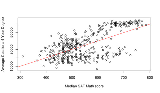
It turns out that as you let the schools be more selective (i.e. select a lower acceptance rate), the correlation becomes stronger. One can especially see this at around the 30% acceptance rate mark, where we have a correlation of around 0.8. An interesting factor one can explore deeper is the financial aid of these “selective” schools as well; I’ve noticed that generally the more selective a school is in the US, the nicer the financial aid program if you’re considered lower class.

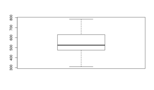
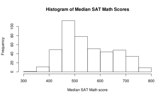
Next, I explored some general information about the Median SAT Math score of these selective schools. It’s interesting to note that the median is around the 525 range. This is around what you would expect for the median score in general, since each person is graded on a range from 200-800. In fact, when checking the entire dataset, we find that the median is at 517, meaning that the “selective” schools in this case don’t really vary much from just all of the schools. One can also notice that the mean of the selective schools is approximately the same as the mean of all of the schools. A boxplot and histogram of the data can be seen below.

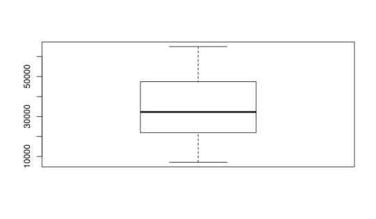
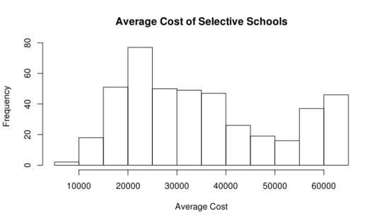
Next, I explored the summary statistics of the cost of selective schools. The median price is around $32,260, which is much larger than the median price for all schools, which is $22,880. This seems to suggest that our definition of selective is appropriate, since a more selective school should cost more. Once again, I would be interested in exploring these figures in relation to the average financial aid package per student at these universities in a future post. Below you can once again see the histogram and boxplot I generated for these figures.

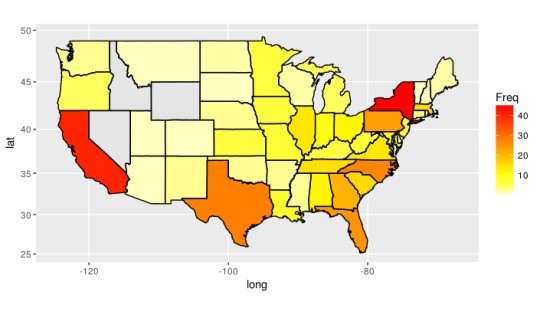
Finally, I wanted to explore the locations of these selective schools. I found that the highest number of selective schools can be found in Virginia, while the lowest number (not accounting for states who have zero selective schools) is Alaska. Interestingly, home state, Indiana, has around 10 schools matching this criteria (putting it on the higher end, which was mildly unexpected). I decided to then develop a heat map of the united states based on the frequency of selective schools. After modifying this post, I was able to do so, and the result can be seen below.

Overall, there were a lot of interesting things going on with this dataset, and I really explored only a few aspects of it in order to get some practice with R. I highly recommend you check it out and play around with it yourself. My code can be found here.

[learning2program]

Hall’s Theorem and an Application to Cards

Today, we’ll work a little bit in graph theory and discuss Hall’s Theorem.

Hall’s Theorem, or what’s sometimes referred to as Hall’s Marriage Theorem, is a theorem which states the following: there is a complete matching on a connected bipartite graph if and only if for every subset A of V_1 we have

$$ |A| \leq |N(A)| $$

where we define N(A) to be the set of all nodes such that there is a node in V_1 that shares an edge with it.

There’s a lot of terminology here, and I recommend in order to better understand it you look at the wikipedia post for Hall’s Marriage Theorem, found here. There is a pretty cool application of this theorem which we’ll explore today. The application is as follows: Given any deck of cards, create 13 piles of four cards taken randomly from the deck. Then one is able to select one card from each pile such that we have all of the cards ranging Ace to King.

In order to play around with this concept, we’re going to need two packages --- the random module, and the networkx module for graph theory. Using these, we are able to construct examples of the application using only four functions. The idea of this is that we generate a deck, randomly place these cards into piles, or in this case into various indices of a dictionary, and then, using the networkx package, we are able to find a complete matching with a little bit of math trickery. The functions are as follows:

check_card(x): This one is just a formatting function. It takes an input of a number, ranging from 0 to 12, and if it’s 0 it returns “A”, if it’s 10 it returns “J”, if it’s 11 it returns “Q”, and if it’s 12 it returns “K”, which correspond to Ace, Jack, Queen, and King respectively.

#return the card value def check_card(x):    if x == 0:        return "A"    if x == 10:        return "J"    if x == 11:        return "Q"    if x==12:        return "K"    return x

generator(): This function takes no input. It generates a list from 0 to 52 which contains four copies of each number from 0 to 12. We then create a dictionary called pile, and for each index from 1 to 13 we randomly select objects from the deck and place them in the index, removing them from the deck list in the process. We then return the pile dictionary when we’re done.

def generator():    #holds the list of cards    list_of_cards = []    #generates the list    for i in range(13):        for j in range(4):            list_of_cards.append(i)    #holds the piles    pile = {}    #adds cards to each pile    for i in range(13):        pile[i+1] = []        for j in range(4):            x = random.choice(list_of_cards)            pile[i+1].append(x)            list_of_cards.remove(x)    return pile

find_complete_collection(pile): This is where the trick comes in. We create a bipartite graph, with the nodes in our first set, V_1, denoting the 13 piles, and the nodes in the second set, V_2, denoting our 13 cards. We draw an edge between a node from V_1 to V_2 if the card denote by the node in V_2 is in the pile corresponding to the node in V_1. Note that this pairing creates the condition necessary for Hall’s theorem; i.e.,

$$ |A| \leq |N(A)|$$

for all

$$A \subset V_1.$$

Then, using the networkx package, we are able to find the maximum_matching and, after formatting it to be a little nicer to deal with, we return it.

#Finds a complete matching def find_complete_collection(pile):    G = nx.Graph()    for i in pile:        G.add_node(i)    for k in range(13, 27):        G.add_node(k)    V1 = []    V2 = []    for i in range(13):        V1.append(i)        V2.append(i+13)    for i in V1:        for j in pile[i+1]:            G.add_edge(i, j+13)    z= nx.bipartite.maximum_matching(G)    listing = {}    for i in range(13):        listing[i] = z[i]    return listing

check_halls(coll): Here, we simply check the condition that there is a complete matching. In other words, we check that every pile appears once, and every card appears once.

def check_halls(coll):    #first, check if all of the piles are used    check = []    for i in range(13):        check.append(i)    for i in coll:        if i in check:            check.remove(i)    if len(check) != 0:        return False    #now, check if all of the cards are used    for i in range(13):        check.append(i)    for i in coll:        if coll[i]-13 in check:            check.remove(coll[i]-13)    if len(check) != 0:        return False    return True

pile_writer(number_of_times): Here, there isn’t much going on. We simply iterate over the number_of_times, and each time we do this we append it to a text file dubbed Card_Piles.txt. We display what each pile has, and also what the complete matching produced by our prior function is.

#outputs it to a text file in a nice format def pile_writer(number_of_times):    text_file = open("Card_Piles.txt", "w")    for k in range(number_of_times):        pile = generator()        text_file.write("Time " + str(k+1) + ":\n")        text_file.write("\n")        for i in range(13):            text_file.write("Pile " + str(i+1) +":\n")            strng = ""            for j in pile[i+1]:                strng += str(check_card(j))                strng += ", "            strng2 = ""            for i in range(10):                strng2 += strng[i]            text_file.write(strng2 + "\n")        text_file.write("\n")        text_file.write("Complete collection: " )        gh = find_complete_collection(pile)        strngg = ""        for z in gh:            strngg += str(check_card(gh[z] - 13))            strngg += str(" from ")            strngg += "Pile "            strngg += str(z+1)            if z == 12:                strngg += " "            else:                strngg += ", "        text_file.write(strngg)        text_file.write("\n \n")        text_file.write("Is there a complete matching?")        if check_halls(gh) == True:            text_file.write(" Yes")        else:            text_file.write(" No")        text_file.write("\n \n")

I ran it for around 10 times, and in the Github is the text file of what was produced. Notice that every time we have a complete matching, regardless of how we randomly chose the piles. This matches the theorem that is established by Hall.

To see the code for yourself, you can find it here. To see the corresponding text file, you can find it here.

[learning2program]

Tweet Scraping

Today, we’ll be scraping tweets.

First, I’d like to thank the user Yanofsky on Github for the inspiration for the project. Much of the work here was thanks to him, and he really should take the credit. What I created was really a slight modification of his code.

We’ll just be doing a basic scrape of a users Tweets and saving them into a text file. First, we’ll need to acquire a few keys. If you don’t have a Twitter account, it is a requirement to have one in order to use the Twitter API, which is called Tweepy. See the link for more on the documentation of Tweepy.

Once you’ve made your Twitter account, you’ll go to https://apps.twitter.com and create an app. Select a name for your app (it doesn’t really matter what for our purposes) and then create the app. You’ll want to find four different keys --- the consumer key, the consumer secret key, the access token, and the access secret token. Save those somewhere safe, or keep the tab open for quick reference.

Now, we start actually coding. You’ll want to first import two things:

import tweepy from tweepy import OAuthHandler

After importing those two things, save your keys in the following variables where the empty quotations are:

consumer_key = '' consumer_secret = '' access_token = '' access_secret = ''

Then, with all of that saved, we load up the following code:

auth = OAuthHandler(consumer_key, consumer_secret) auth.set_access_token(access_token, access_secret) api = tweepy.API(auth)

and now we have access to the API using the api prefix on our code! See the documentation link for more information on what you can do with tweepy.

There’s only one function in the script, called the save_tweet function.

save_tweet(screen): The save tweet function takes only one parameter, which is the screen name. Note that this is the username of the person you wish to pull the tweets of, and it must be in a string (so wrap it in quotations). We start by initializing an empty list called tweets. We then initialize a new list called new_tweets which will hold the temporary tweets that we call each time. We then use the function api.user_timeline, with the parameters screen_name = screen and count = 200. Hypothetically, we would like to set count to be arbitrarily high so that it pulls all of the tweets, however the function caps out at 200 tweets per call. So, we start by calling the initial 200, and then we extend our tweets list by this new_tweets. Under a variable called maxdate, we save the last date called (which is found by using tweets[-1].id-1). Then, we start a while loop. Within the while loop, we add a new parameter to api.user_timeline --- we set max_id = maxdate. We essentially do everything we just did before, except we update the maxdate variable to the most recent date. The while loop terminates when new_tweets has length 0.

We then create another list, called savetweets. Here, we’ll have the actual text of the tweets that we’re saving. We run a for loop for each item in tweets, appending to savetweets the text of the tweet in tweets (say that three times fast). We then finish up the script by opening a text file, and for each tweet in savedtweets we write the tweet on a new line. We terminate the script by closing the text file.

def save_text(screen):    #an empty list to hold a list of objects    tweets = []    #pulls the initial 200 tweets (max)    new_tweets = api.user_timeline(screen_name = screen, count = 200)    #gets the last date that was retrieved    maxdate = new_tweets[-1].id - 1    print('init')    #extends the list adding the newtweet objects    tweets.extend(new_tweets)    while len(new_tweets) != 0:        #pulls the next 200 tweets        new_tweets = api.user_timeline(screen_name = screen, count = 200, max_id = maxdate)        #extends the list again        tweets.extend(new_tweets)        #gets the next maxdate        maxdate = tweets[-1].id - 1        #lets the user know how far along we are        print('loaded ' + str(len(tweets)) + ' tweets so far')    print('finished loading!')    #this is the actual text    savetweets = []    #for i in the tweets list, pull the text and save it in a new list    for i in tweets:        savetweets.append(i.text)    print('now saving it to a text file...')    #open a file    text_file = open(str(screen) + "_tweets.txt", "w")    #write the tweet on a new line    for i in savetweets:        text_file.write(i + "\n")    #close the file    text_file.close()    print('finished!')

The script can be found here, and the test text file can be found here.

[learning2program]

The Fibonacci Sequence

Today, we’ll be doing various things with the Fibonacci sequence.

The Fibonacci sequence is probably the sequence which inspired me to go into math. When I first heard about it, I was absolutely blown away by two things --- first off, how simple it is to understand the sequence (just add the last two things in the sequence to get the next) and second, how prominent it was in the weirdest of places. For example, it comes up in things like the growth of sunflowers, the reproduction of rabbits, and in the tattoos of hipsters everywhere (I admit, at one point I wanted to get a Fibonacci spiral tattoo on myself as well). Nevertheless, it imparted onto me that even simple things have powerful impacts in the field of mathematics, and it’s what pushed me to do what I do today.

I figured that this sequence’s simplicity coupled with it’s power makes it a somewhat important topic to talk about. So today I figured we’ll play around a little bit with the Fibonacci sequence and see what we can do. With slight modification, I’m pretty sure you can solve one of the earlier Project Euler problems. Let’s dive into a few things, though.

Off of the top of my head, there are three (technically maybe two) major ways of tackling the problem of generating Fibonacci numbers. The first is with using lists. The pro is that this is very easy to visualize in ones head --- like I said earlier, to find the next value, we take the last two and add them together. The con to this approach is that it is very memory intensive. For example, I tried to run it on 4,000,000 (*hint* to those who want to try the Project Euler problem) and it crashed my computer almost immediately. However, this approach does have it’s advantages; it lets one see what’s going on at each iteration of the process. The second approach is by using recursion, which Python is relatively bad with. The third is by using a somewhat memoryless property that the Fibonacci sequence carries with it. Memorylessness is something that those with experience in Probability should be experienced with --- it means that we only care about the last finite sequence of things that happened, rather than caring about the whole (I’m being somewhat loose with my definition of memorylessness; it technically has a more strict definition, which one can see in the wikipedia article. My definition of memorylessness is useful in establishing the heuristic for which we will build our function with). For this example, we only care about the last two things, and the rest of it doesn’t matter for us. Using this, we are able to bypass the memory problem that was mentioned earlier. Let’s jump in.

fib(start1, start2, number_of_elements): This function takes what I would consider to be the standard three parameters for a Fibonacci function that does not utilize recursion. We give it two things for which our list (which in our function is denoted lis) will start with, and from there we will build the rest of the list. So for example, if we gave it 1 and 2 as it’s starting point, it will generate the list to be

lis = [1,2].

Next, it will take the last two elements in the list --- python uses lis[-1] to find the last element in a list, and lis[-2] to find the second to last element. So, we append this to the list:

lis.append(lis[-1]+lis[-2]).

We have this wrapped within a while loop which at each iteration checks the length of the list. If the length of the list has exceeded number_of_elements-1, then the while loop terminates, and the function returns the list generated.

In our practice case of fib(1,2,10), we see that it outputs [1, 2, 3, 5, 8, 13, 21, 34, 55, 89], as expected.

def fib(start1, start2, number_of_elements):    # we start with the first two elements of our list    lis = [start1, start2]    # while our list is less than our desired length, we add the last two elements in the list and append it to the list    while len(lis) < number_of_elements:        lis.append(lis[-1] + lis[-2])        # return list return lis

So, we now have the list of Fibonacci numbers. Let’s next inspect some properties of the Fibonacci numbers.

find_even(lis) (and likewise, find_odd(lis)): This function just finds all of the even elements of a list and returns them. There’s nothing really too fancy here.

def find_even(lis):    # generate an empty list to store all of the elements    lis2 = []    # for all of the elements in the list, we find the ones that are congruent to 0 mod 2 and append them to the new list    for i in lis:        if i % 2 == 0:            lis2.append(i)            # return the new list return lis2

Using these two functions, we can see whether or not there are generally more even or odd integers for Fibonacci numbers. The reader is encourged to think about this question before reading.

To test this, we inspect the first 10, then 50, then 100 elements. One can note that the ratio of evens to odds is around 1 : 2. The first observation is that there must always be more odds than evens if we start at 1,2. Note that this is not really a formal proof, but rather an illustration of what is going on in the relation of evens to odds. This fact follows by the basic property of numbers --- an even plus and odd number is odd, an even plus an even is even, and an odd plus an odd is even. So, we have that 1,2 is odd, 2,3 is odd, and 3,5 is even, but then 5,8 is odd, and so on. The sequence can then be generalized to be

$$[1,0,1,1,0,1,1,0,1,1,...]$$

where {1,0} denotes the congruent classes modulo 2. So, we can always expect there to be more odds than evens. In fact, assuming an infinite number of elements, the probability of randomly selecting an odd number should be 2/3.

So, we’ve found an interesting relation between the odds and evens of the Fibonacci sequence. However, I promised earlier a way to calculate higher Fibonacci numbers, since, as I mentioned, this is extremely ineffective when calculating anything beyond a million (and will in fact crash your computer). I also mentioned Python is bad at recursion. This does not mean that one cannot use recursion; there are plenty of examples all around the internet of doing the Fibonacci sequence using recursion in Python. It just means that the more Python way of doing things is to use some sort of loop to find the next value.

high_fib(start1, start2, number_of_elements): I kept the parameters to be roughly the same as prior since we have a familiarity with them. We begin our Fibonacci sequence at start1 and start2 per usual, and go all the way up to where number_of_elements is (which denotes the last value in our Fibonacci list from the prior function). We first, for clarity, create two variables called first and second. First will hold the smaller value while second will hold the largest. In a while loop, we have the following procedure. We start by assigning second to a temporary variable for now. Then, we assign to second the summation of first and second. We then assign to first the temporary variable, and finish by increasing our counter variable (which measures whether or not we’re above number_of_elements). We then finish the function by returning second, or the last value generated.

def high_fib(start1, start2, number_of_elements):    # the count starts at 2 since we have the first two elements in our list already (customarily 1,2)    # should be modified based on where you're starting though    count = 2    # one should probably just use start1 and start2, but I figured it would be easier to read if I used first and second    first = start1    second = start2    # this should look familiar    while count < number_of_elements:        # temp holds our temporary value, since we'll erase it momentarily        temp = second        # replace second by the sum        second = first + second        # replace first by temp        first = temp        # increase our counter        count += 1        # return the final value return second

Using the same test case as prior, we have high_fib(1,2,10) returns 89, as expected.

Note that high_fib can retrieve large values from the Fibonacci list without consuming as much memory as the prior function. It’s rather a matter of time instead of memory.

Using the philosophy from this lesson, one can most likely solve the Project Euler problem from earlier. In fact, I encourage the reader to do so, since it’s good practice. Like always, you can find the program on the Github page for the blog.

I’d like to finish off by apologizing for the lack of content last week. It was midterms time, so I had to focus on school instead of producing stuff for this. I should be making more interesting content this week.

[learning2program]

Catterplot

Today, we will be doing a fun little project -- playing around with the catterplot feature in R.

I saw the catterplot library and realized I needed to do something right away with cats, but what exactly? If you haven’t seen the catterplot library yet, check it out on github here. It’s probably one of my favorite useless R libraries next to the ubeR library --- for when you’re so lazy you have to order an ubeR from your console.

Obviously, if you have something that plots catterplots, you need to use cat data to play around with it. A quick google search leads me to this convenient cat data on cat weight vs. their heart weight which will be perfect for the catterplot. Below is the code used to generate our catterplot:

install.packages('devtools') library(devtools) install_github("Gibbsdavidl/CatterPlots") library(CatterPlots) install.packages('boot') library(boot) dogscats <- catplot(catsM$Bwt, catsM$Hwt, size=0.1, catcolor=c(0.7,0.7,0.7,1),                    cat=11,                    xlab="Body Weight",                    ylab="Heart Weight",                    main="Cat Body Weight vs. Heart Weight")

and here is the catterplot generated:

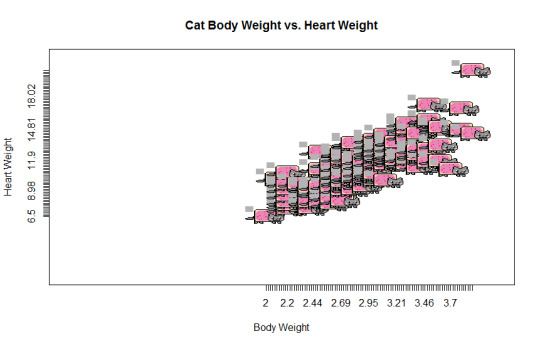
I seem to be having a mild problem with the scaling on my catterplot. I’ll update this if I ever figure it out. But I figured amidst all of the math-y posts, this would be a good filler, and also a good lead in to doing more R related stuff instead of just Python.

[learning2program]

Interesting fact about the GCD

Today, we will be utilizing the Euclidean algorithm module we wrote earlier to study an interesting fact about GCD.

I learned a cool new fact today that I thought I’d share. It uses the Euclidean algorithm module that I wrote up earlier like I said, so if you haven’t see that yet you should read it here.

Today we will be studying the fact that

\[\sum_{\substack{1 \leq a \leq n\ gcd(a, n) =1}} a = \frac{n \phi(n)}{2}. \]

I’ll first cover some preliminaries though. First, one should know what I mean when I say

\[ \phi(n). \]

This is known as the Euler totient function, and is an interesting function in number theory. It counts the number of numbers coprime to your input which are less than your value. It has a variety of applications and a long history behind it which is outside the scope of this post, but you can see more here.

Next, we’ll need a theorem.

Theorem: If gcd(a, n) = 1, then gcd(n-a, n) = 1.

Proof:

By Bezout's Identity, we have that gcd(a, n) = 1 implies

\[ \alpha a + \beta n = 1.\]

Add and subtract alpha n to the left hand side to get

\[ \alpha a + \beta n - \alpha n + \alpha n = 1.\] By simple algebra, we get

\[ \alpha(a - n) + n(\beta + \alpha) = 1.\]

Let

\[ \gamma = \beta + \alpha\]

for notational simplicity. Then we have that

\[ \alpha(a-n) + n\gamma = 1.\]

By the converse of Bezout's Identity, this then gives us

\[\gcd(a-n, n) = 1.\]

However, note that

\[\gcd(-(a-n),n) = \gcd(a-n, n)\]

(this follows since if d | m, n then d | -m, n; so we have that (-m,n) and (m,n) have the same set of common divisors, which implies the same gcd), which then implies gcd(n-a, n) = 1. Q.E.D.

Using these two, the construction of the earlier claim is rather clear. We can use an argument similar to that of Gauss when counting the integers. Let

\[x_1, \ldots, x_{\phi(n)} \]

be the integers which are coprime to n in ascending order. Then we can arrange the integers to then be

\[ x_1, \ldots, x_{\phi(n)} \]

\[ x_{\phi(n)}, \ldots, x_1. \]

Add the integers vertically to then get $\phi(n)$ instances of n. This is clear from the theorem earlier. We however have added the sequence to itself, and so dividing it by two then gives us the sum of the coprime integers. Therefore, we have

\[\sum_{1 \leq a \leq n, gcd(a, n) =1} a = \frac{n \phi(n)}{2}. \]

One can then check this for the first however many integers using python. For simplicity, I will be only checking the first 30 integers; however, you can modify the file to be as large as you want (it will probably start slowing down a lot as you set the integer amount to be higher and higher, however). There is really only one function that we will be doing to use this, though we will import the gcd function from our euclideanalg module.

check(p): The function starts by constructing a list of all of the positive integers less than p which are coprime to p. Here, we use the gcd function to check if gcd(i, p) == 1 at each iteration of i. Next, we sum up each of the numbers in this new list that we’ve constructed and save it in a variable denoted sum. We take the length of the list (which is equivalent to the Euler totient of p) and then calculate the value

\[\frac{n \phi(n)}{2}. \]

If the sum of the coprimes and this value are equivalent, the function returns true; otherwise, the function returns false (however, by the prior claims, we have shown that this should never return false). We now have a tangible way to view whether or not this claim is true! The code for the function follows

def check(p): print('checking ' + str(p)) primes = [] for i in range(1, p): if gcd(p, i) == 1: primes.append(i) sum = 0 print('coprimes: ' + str(primes)) for i in primes: sum += i print('sum of coprimes: ' + str(sum)) #now to actually check tot = len(primes) print('euler totient function: ' + str(tot)) total = (p * tot)/2 if total == sum: return True else: return False

As always, you can find this on the github page here.

[learning2program]

Iterative Methods for Finding Eigenvalues

 Today, we will be reviewing some iterative methods for finding eigenvalues.

Recall that the definition of an eigenvector/eigenvalue is given some linear transformation,

\[T :  (V/F)^n \to (V/F)^n \]

then v is an eigenvector of T if T(v) is a scalar multiple of v. In other words, if we have

\[ T(v) = \lambda v, \lambda \in F. \]

Eigenvalues and eigenvectors are extremely useful in applications. For example, Google’s pagerank algorithm uses eigenvalues and eigenvectors to rank websites according to their relevance to your search. They also have uses in dynamical systems and differential equations. A good math overflow topic post about this can be found here.

In some cases, however, knowing an eigenvalue or eigenvector exactly isn’t quite that useful, since finding it generally involves using the characteristic polynomial of a matrix. Instead, in order to find quick results, it’s much more useful to estimate these things. We will be discussing the power method, the inverse iteration method, the shifted inverse iteration method, and the Rayleigh Quotient iteration method in order to find (relatively) fast estimates of eigenvalues, which will be relevant in a future project on Google’s pagerank.

In order to preform these operations, we will be utilizing the Python package SymPy for matrices. More details about this can be found here. I chose SymPy mostly just to practice with non-Numpy libraries, although Numpy can also probably be used for this. I would actually recommend that if you’re going to try to code this on your own to use Numpy, since I believe they have optimized their library using C, meaning it will be faster than what I’ve done (I have no clue if SymPy has done this, so this statement might be false). We also use the default math package.

As a preliminary, we create a norm function.

norm(vector): This function starts with a variable called norm_sq set at 0. It then iterates through all of the values of the vector, squaring them and adding them to norm_sq. It then returns the square root of norm_sq.

def norm(vector):    norm_sq = 0    for j in vector:        norm_sq += j * j    return math.pow(norm_sq, 0.5)

Power Method:

We first need to discuss a preliminary result.

Theorem: (Rayleigh Quotient) If v is an eigenvector of a matrix A, then its corresponding eigenvalue is given by

\[ \lambda =  \frac{Av \cdot v}{v \cdot v}.\]

Proof: Since v is an eigenvector of A, we know that by definition

\[Av = \lambda v \]

and we can write

\[\frac{Av \cdot v}{v \cdot v} = \frac{\lambda v \cdot v}{v \cdot v} = \frac{\lambda(v \cdot v)}{v \cdot v} = \lambda, \text{   Q.E.D.} \]

Given an n by n matrix, denoted by A, consider the case where A has n real eigenvalues such that

\[|\lambda_1| > |\lambda_2| > \cdots > |\lambda_n|. \]

Assume that A is diagonalizable. In other words, A has n linearly independent eigenvectors, denoted

\[x_1, \ldots, x_n \]

such that

\[Ax_i = \lambda_i x_i, \text{ for i = 1,..,n} \]

Suppose that we continually multiply a given vector by A, generated a sequence of vectors defined by

\[x^{(k)} = Ax^{(k-1)} = A^kx^{(0)}, \text{ }k=1,2,... \]

where 0 is given. Since A is diagonalizable, any vector in Rn is a linear combination of the eigenvectors, and therefore we can write

\[x^{(0)} = c_1x_1 + \cdots + c_nx_n. \]

We then have

\[ \lambda^k_1 \bigg[ c_1x_1 + \sum_{i=2}^nc_i\bigg( \frac{\lambda_i}{\lambda_1}\bigg)^k x_i\bigg].\]

Note that we assumed that the eigenvalues are real, distinct, and ordered by decreasing magnitude. It then follows that the coefficients of the xi’s converge to zero as we let k go to infinity. Therefore, the direction of x(k) converges to that of x1. Once we have the eigenvector from the power method, we can use the prior defined Rayleigh Quotient to find the eigenvalue as we wanted.

Using this, we then have an algorithmic way to find eigenvalues, and so we are able to code this.

powermeth(A, v, iter): Here, we have three input variables. A denotes our matrix, as should be expected by prior notation, v denotes our start vector, and iter represents the number of iterations this runs for. The function starts by running a for loop, and solving the equation

\[w = Av^{(k-1)} \]

for w. SymPy conveniently does matrix multiplication, and so all we have to do is multiply as though they were integers. We then find the norm using the norm function, as defined prior, and assign it to nor. At the end of every iteration, we find the next v vector by normalizing w (i.e. dividing tmp by nor). The function then terminates by returning the eigenvalue, which was the last value assigned to nor.

def powermeth(A, v, iter):    for i in range(iter):        #create a temporary vector to hold v^(1)        tmp = A * v        #find norm        nor = norm(tmp)        #normalize v for next iteration; i.e. v/||v||        v = tmp/nor    #returns a tuple: v is the eigenvector, nor is the eigenvalue    return nor

There are some downsides to this method, however. First off, it only finds the eigenvalue with the largest magnitude. In addition, we see that convergence is ensured if and only if all the eigenvalues are distinct. The convergence also depends on the difference of magnitude between the largest eigenvalue and second largest eigenvalue --- if they are close in size, then convergence is slow. Despite these drawbacks, though, the power method is extremely useful and still used in algorithms today.

Inverse Iteration Method:

If we have an invertible matrix, A, with real nonzero eigenvalues

\[\{\lambda_1, \ldots, \lambda_n \}, \]

then the eigenvalues of A^(-1) (A inverse) are

\[\{1/\lambda_1, \ldots, 1/\lambda_n \}. \]

In other words, by the theory of the power method, we can note this gives us the smallest eigenvalue, as opposed to the largest. The function is then as follows.

inverse_iter(A, v, iter): The requirements are the same as for the power method. The only difference is that at the start of the function, we have to calculate the inverse of A. To do this, we use SymPy’s inverse function, which uses Gaussian-Elimination to find the inverse. The process is then the same, substituting the inverse for A at each instance.

def inverse_iter(A, v, iter):    #Save time on calculation by doing the inverse first, instead of every iteration    B = A.inv()    for i in range(iter):        tmp = B * v        #find norm        nor = norm(tmp)        #normalize        v = tmp/nor    #returns the eigenvalue    return (1/nor)

The observant reader will then notice that this is a much more robust method than the prior power method. The reason for this is that we can adept this method to find any eigenvalue of the matrix, assuming we know a close estimate. Note that for any real number, the matrix

\[B = A - \mu * I \]

has eigenvalues

\[ \{\lambda_1 - \mu, \ldots, \lambda_n - \mu \}. \]

In particular, by choosing our real number to be close to the eigenvalue we want, we have that this will be the smallest eigenvalue and so by the inverse iteration method we can find it. The function is then as follows

inverse_iter_shift(A, v, estimate, iter): The difference is now we take an estimate. We start by finding I using SymPy, multiplying our estimate to I, and then subtracting I from our initial matrix A. The process is then the same as for the inverse iteration method. This is because we transformed our matrix accordingly, and so by definition the eigenvalue is also transformed.

def inverse_iter_shift(A, v, estimate, iter):    #since we asume the matrix to be square    I = sympy.eye(A.shape[0])    #Shift the matrix    B = A - I*estimate    #Invert first    B = B.inv()    for i in range(iter):        tmp = B * v        #find norm        nor = norm(tmp)        #normalize        v = tmp/nor    #returns the eigenvalue    return (1/(-nor) + estimate)

Rayleigh Quotient Iteration:

What if we could change the shift in the inverse_iter_shift function so that it adapts each iteration? We would have much faster convergence doing so. In fact, there is a method to do this using the Rayleigh Quotient Iteration. Here, we pick a starting vector, and calculate our estimate by preforming the operation

\[\lambda^{(k)} = (v^{(0)})^T A (v^{(0)}). \]

Thus, it is the same as for the inverse_iter_shift except we preform this calculation at every iteration. While more expensive, it has a cubic convergence rate as opposed to linear, and we don’t need to “know” an estimate (it depends instead on our selection of the initial vector).

RQI(A, v, iter): It essentially follows by prior, except we have to initialize a unit matrix I using SymPy to multiply with lambda. We also solve

\[(A - \lambda^{(k-1)}I)w = v^{(k-1)} \]

for w. Note that the lambda are our eigenvalues in this instance.

The code is then as follows.

def RQI(A, v, iter):    #Since we assume the matrix to be square    I = sympy.eye(A.shape[0])    for i in range(iter):        # Find lambda_0 (denote it lam)        lam = sympy.Transpose(v) * A * v        lam = lam[0]        B = A - I * lam        #If it converges, then the matrix may not be invertible (?)        try:            tmp = B.inv() * v        except:            break        #find norm        nor = norm(tmp)        #normalize        v = tmp/nor    return lam

The code can be found at the Github page, per usual. Credit to Maysum Panuj for the pseudocode inspiration.

[learning2program]

Z-Value, T-Value, Confidence intervals

Today, we will be finding Z-values, T-values, and confidence intervals.

This is rushed again. I apologize for the lack of non-rushed content lately, I’ll be back to normal after these next two weeks.

Z-values and T-values are important concepts for statistics. They are used to determine the likelihood that about a parameter of a statistic is true or not. For example, if we were given a collection of data, and wanted to find the likelihood that the true mean was

\[\mu = \mu_0 \]

we would want to find the p-value of said hypothesis. While the p-value does not actually confirm or deny the hypothesis, it does give evidence as to whether or not the claim is true. For example, if we have a large p-value, then it’s probable that the claim is true; on the other hand, if we have a small p-value, then it’s less likely the claim is true. The reasoning for this is that we can imagine our data as a normal distribution (especially if we have a large amount of data – see central limit theorem). The p-value then denotes the distance from our hypothesis to the sample mean. If this distance is not far, then it’s likely that this could be our true population mean; however, if the distance is far, we would expect this to not be the case, since if we had such a large amount of data we’d expect the sample mean to approach the true mean.

Note that the difference between the t-value and the z-value is that the t-value only uses the sample variance, while the z-value requires knowledge beforehand of the true variance. As you would expect, it’s unlikely we would know the true variance in the real world, and so the t-value is most often used in real world experiments.

To use this module, we will utilize our correlation package that was written earlier. If you haven’t seen that article, see here. The packages that will be used are the math package, and the scipy.stats package (in order to find the norm cdf and the t-value).

tpvalue(mu0, xbar = False, s=False, n=False, data=False): This finds the t-value. Note that you can either manually plug in the xbar, s, and n values, or instead plug in a vector of data. If you give it a vector of data, it uses the correlation package to find the sample mean, sample variance, and the size of the data. It then uses the scipy package to find the t-value, assigning it to the variable c, and then solves the formula

\[P_{\mu_0, \sigma^2} \bigg( |T| \geq \big|\frac{\bar{x}-\mu_0}{s/\sqrt{n}} \big| \bigg) = 2 [1- c]. \]

It then returns the corresponding p-value.

def tpvalue(mu0, xbar = False, s=False, n=False, data=False):    if (s == False or n==False or xbar == False) and data==False:        return None    if data != False:        n=len(data)        s = math.pow(variance(data), 0.5)        sqrtn = math.pow(n, 0.5)        xbar = mean(data)        t = abs((xbar-mu0)/(s/sqrtn))    else:        sqrtn = math.pow(n, 0.5)        t = abs((xbar - mu0)/(s/sqrtn))    return 2*(1-st.t.cdf(t, n-1))

zpvalue(mu0,variance,xbar = False, n = False, data = False): This is the Z-value analogy to the tpvalue function. Note that everything is essentially the same, except that we now must plug in the true variance. It then uses the scipy package to find the corresponding z-value, and solves the analogous equation to prior.

def zpvalue(mu0,variance,xbar = False, n = False, data = False):    if (xbar == False or n == False) and data == False:        return None    if data != False:        n = len(data)        sqrtn = math.pow(n, 0.5)        xbar = mean(data)        sigma = math.pow(variance, 0.5)        z = abs((xbar-mu0)/(sigma/sqrtn))    else:        sqrtn = math.pow(n, 0.5)        sigma = math.pow(variance, 0.5)        z = abs((xbar - mu0)/(sigma/sqrtn))    return 2*(1-st.norm.cdf(z))

tconfident(siglev, n= False, xbar = False, s = False, data = False): This is similar to the tpvalue equation, except we now need to input the significance level. Once we have the significance level (denote it by gamma), we then must solve

\[t_{(1+ \gamma)/2, n-1}, \]

where n is the size of the vector. Note that the t function finds the inverse t-value corresponding to

\[(1+ \gamma)/2 \]

given n-1 degrees of freedom. It then solves the equation

\[\bar{x} \pm t_{(1+ \gamma)/2, n-1}\sqrt{\frac{s^2}{n}} \]

and returns a tuple of the form (lower bound, upper bound).

def tconfident(siglev, n= False, xbar = False, s = False, data = False):    if (s== False or n==False or xbar == False) and data == False:        return None   ��if data != False:        n = len(data)        sqrtn = math.pow(n, 0.5)        s = math.pow(variance(data), 0.5)        xbar = mean(data)    else:        sqrtn = math.pow(n, 0.5)    inv = (1+siglev)/2    c = st.t.ppf(inv, n-1)    lowbound = xbar - c * (s/sqrtn)    upbound = xbar + c * (s/sqrtn)    return (lowbound, upbound)

zconfident(variance, siglev, n = False, xbar = False, data = False):

Once again, this is the z-value analogy of tconfident. This time, instead of solving the t function, we instead solve

\[z_{(1+ \gamma)/2}, \]

which is the inverse cdf of the normal distribution N(0,1) at

\[ (1+ \gamma)/2.\]

Using this, it solves the equation

\[\bar{x} \pm z_{(1+\gamma)/2} \sqrt{\frac{\sigma^2}{n}} \]

and returns a tuple of the form (lower bound, upper bound).

def zconfident(variance, siglev, n = False, xbar = False, data = False):    invs = (1 + siglev)/2    c = st.norm.ppf(invs)        if (xbar == False or n == False) and data == False:        return None    if data != False:        n = len(data)        sqrtn = math.pow(n, 0.5)        xbar = mean(data)    else:        sqrtn = math.pow(n, 0.5)    sigma = math.pow(variance, 0.5)    lowbound = xbar - c*(sigma/sqrtn)    upbound = xbar + c*(sigma/sqrtn)    return (lowbound, upbound)

findn(siglev, leng_of_int, variance):

This finds the amount of samples one must take in order to get the corresponding length of interval at the given significance level. For example, if we were to flip a coin and observe the proportion of heads on a single toss, how many times must we toss the coin in order to have an interval of length less than 0.1? Note that this is the distribution Bin(theta, n) and so we have that

\[Var = \theta(1-\theta). \]

In order to find the number of times, we then need to solve the equation

\[z_{(1+ \gamma)/2} \frac{\sigma_0}{\sqrt{n}} \leq l \]

where l is the length of the interval. Solving for n, we get

\[n \geq \sigma_0^2 \bigg(\frac{z_{(1+\gamma)/2}}{l} \bigg)^2. \]

Thus, using the formula (or the function), we find that n must be at least 97 times.

Note that the function returns the ceiling, or the closest integer greater than the value, of

\[ \sigma_0^2 \bigg(\frac{z_{(1+\gamma)/2}}{l} \bigg)^2\]

since it does not make sense to have a fraction of a toss.

def findn(siglev, leng_of_int, variance):    invs = (1+siglev)/2    c = st.norm.ppf(invs)    return math.ceil(variance/(math.pow(leng_of_int/c, 2)))

As I posted earlier, you can now find the code on the github. Here is the link.

[learning2program]

Github page

I’ve moved to an official github page! It can be found here.

[learning2program]

Finding correlation

Today, we’ll be finding the correlation between two vectors of information.

With midterms coming up, I decided to do another light bit of coding. Since midterms are coming up, I’ll probably be doing a lot of “lighter” projects until afterwards, when I can start doing some more involved things.

Correlation is an important thing in statistics. While correlation does not imply causation, it is an important factor in judging whether two vectors of information are related to each other. The most common way to calculate correlation between two vectors is to use Pearsons correlation coefficient, which is what we will be doing today. In order to find this, one needs to know the mean of the vector, the variance, and finally the covariance. The equation for correlation is

\[\rho_{x,y} = \frac{cov(X,Y)}{\sigma_x\sigma_y},  \]

where sigma is the standard deviation (the square root of the variance).

Note that this does require the math library, which I believe is imported with Python.

mean(list): This one is similar to what we did in our linear regression module. We have

\[\bar{x} = \frac{1}{N} \sum_{i=1}^N x_i, \]

where N in this case is the length of the vector. We utilize a for loop and sum over all of the values.

def mean(list):    x = 0    for i in list:        x+=i    return (x/len(list))

variance(list): We have to calculate the sample variance. As a fun aside, there are actually multiple definitions for the sample variance -- the one we will be using is the one which gives us an unbiased estimator, i.e.

\[s^2 = \frac{1}{N-1} \sum_{i=1}^N (x_i - \bar{x})^2. \]

The rest of the code is fairly straightforward.

def variance(list):    x = 0    xbar = mean(list)    for i in list:        x += math.pow((i - xbar),2)    #So that s^2 is an unbiased estimator    return (x/(len(list)-1))

covariance(list1, list2): The covariance is a little less straightforward than the last two. Generally, one uses the definition

\[Cov(X,Y) = E(XY) - E(X)E(Y), \]

however since we’re programming this just using the classic definition of

\[Cov(X,Y) = \frac{1}{N} \sum_{i=1}^N (x_i-\bar{x})(y_i - \bar{y}) \]

for discrete random variables is much more straightforward.

def covariance(list1, list2):    #assumes the lists to be of equal length    if len(list1) != len(list2):        warnings.warn("lists need to be of the same length")    x = 0    xbar = mean(list1)    ybar = mean(list2)    for i in range(len(list1)):        x += (list1[i] - xbar) * (list2[i] - ybar)    return (x/(len(list1) - 1))

correlation(list1, list2): The meat of the program, we once again use the formula

\[\rho_{x,y} = \frac{cov(X,Y)}{\sigma_x\sigma_y},  \]

which we now have calculated all the parts for, and plug in the corresponding values.

def correlation(list1, list2):    if len(list1) != len(list2):        warnings.warn("lists need to be of the same length")    covar = covariance(list1, list2)    stdx = math.pow(variance(list1), 0.5)    stdy = math.pow(variance(list2), 0.5)    return covar/(stdx * stdy)

As a test case, we find the correlation between S&P 500 returns and economic growth from here, and note that the program does actually give us the correct value. The code can be found here.

[learning2program]

Finding The Automorphism Group

Another short post. We will be discussing finding the automorphism group for the cyclic group of size n.

Recall that the finite automorphism group is a group of functions from a set X to itself which form a group under compositions of morphisms. One can see from the wikipedia page that this clearly fulfills all of the axioms of a group. As an aside, the automorphism group is also referred to on occasion as the symmetric group on n.

This script specifically focuses on the cyclic group of integers of size n. Since all automorphisms of the cyclic group of integers of size n are defined by left multiplication, i.e.

\[\phi_a(x) = ax \]

then it should be clear that we have

\[Aut(\mathbb{Z}_n) \cong U(n) \]

where here U(n) denotes the group of units (i.e. the elements in Zn which have multiplicative inverses). Note that an element in Zn has a multiplicative inverse if and only if it is coprime to the size of the set.

In order to do this, we will need to find the gcd. Thus, we must utilize a prior module we’ve developed, the Euclidean Division algorithm module (see: here). Therefore, we will first import it. We then only have two functions:

find_automorphism(n): For the integers from 1 to n (we can already exclude 0 since it doesn’t have a multiplicative inverse), we determine whether or not gcd(i, n) = 1. If it does (i.e., it’s coprime to n) then we know it must be in the automorphism group. If it isn’t, we pass over it. We then return the list.

def find_automorphism(n):    list = []    for i in range(1, n+1):        if ea.gcd(n, i) == 1:            list.append(i)    return list

find_size_of_automorphism(n): This simply compiles the list and finds the size.

def find_size_of_automorphism(n):    return len(find_automorphism(n))

Thus, we are now able to construct the group U(n) without having to do any work.

The code can be found here.

[learning2program]

Linear Regression

Today, we will be covering linear regression and coding up a program which does simple linear regression.

Linear regression is one of the fundamental concepts in statistics. It has a plethora of uses, ranging from machine learning to economics to finance to even epidemiology (see: determining a correlation between lung cancer and smoking cigarettes). It’s importance is derived from how useful it is in modeling the relationship between a scalar dependent variable and, in general, one or more explanatory variables. Moreover, it gives one an idea on how to predict the outcome of certain events given a set of data, provided the data lies in a linear fashion.

What I ended up coding today was only simple linear regression. In the real world, one wants to model more than one explanatory variable. However, without going into matrices and developing a matrices module, which I plan on doing later, I will instead have to be relying on the structure of lists. Because of the niceness of two variable linear regression, we end up getting a closed formula for our two coefficients, which I will be abusing in the code.

The general formula for simple linear regression is as follows:

\[ y = x \beta + \epsilon, \text{ }\epsilon, \beta \in \mathbb{R}. \]

In other words, one can imagine the beta and epsilon to be the slope and y-intercept of a linear formula, respectively.

One can technically derive the closed formulas for the beta and epsilon using the least squares estimates, but I won’t be doing that here. For more information on that, see here. Instead, I’ll just be going over what my code does. To see the closed formula for the beta and epsilon, see here.

The code breaks down as follows:

power(x, power): Nothing too crazy here. While there is technically a power function in the math library which probably is much more efficient, for practice I ended up coding up my own. Requires the power to be an integer greater than 0, since inverses will not be considered.

def power(x, pow):    if type(pow) != int and pow > 0:        warnings.warn("pow needs to be an integer value greater than 0")    if pow == 0:        return 1    for i in range(pow-1):        x = x*x    return x

ffsum(list): This function sums up all the elements in a list. Once again, python has a built in function to do this, but for practice I decided to write up my own.

def ffsum(list):    x = 0    for i in list:        try:            x+= i        except:            warnings.warn("you probably don't have just numeric values in the list")    return x

simple_linear_regression(x1, x2): The meat of our rather short script. Here, we create three more lists, dubbed x1x2, x1sq, and x2sq. This is because we’ll need the sums of these lists to find our a and b. Recall from the website that the closed formulas for a and b are

\[ a = \frac{(\sum y)(\sum x^2) - (\sum x)(\sum x y)}{n(\sum x^2)-(\sum x)^2},\]

\[b = \frac{n(\sum x y) - (\sum x)(\sum y)}{n(\sum x^2) - (\sum x)^2}. \]

After finding the sums of x1x2, x1sq (representing x1 squared), and x2sq, it is just a matter of plugging in the numbers. Note that we must preform a type conversion on each of these values into floats instead of ints, so that we get accurate values. Otherwise, the program will round our a and b, which we don’t want.

def simple_linear_regression(x1, x2):    if len(x1) != len(x2):        warnings.warn("the lists are not the same size")    x1x2 = []    x1sq = []    x2sq = []    for i in range(len(x1)):        x1x2.append(x1[i]*x2[i])        x1sq.append(power(x1[i], 2))        x2sq.append(power(x2[i], 2))    #arbitrarily chose x1, could've used x2 as well    n = len(x1)    #Note we have to sloppily convert all of these values to float. Probably should find out a way to do it better.    a = ((float(ffsum(x2))*float(ffsum(x1sq)))-(float(ffsum(x1))*float(ffsum(x1x2))))/(float(n)*float(ffsum(x1sq))-float(power(ffsum(x1), 2)))    b = (float(n)*float(ffsum(x1x2))-float(ffsum(x1))*float(ffsum(x2)))/(float(n)*float(ffsum(x1sq))-float(power(ffsum(x1), 2)))    print('a: ' + str(a))    print('b: ' + str(b))    return a, b

The code can be found here.

[learning2program]

The Euclidean Division Algorithm -- Part 2, Polynomials

Today, we’ll be doing the Euclidean Division Algorithm again, except this time for polynomials!

If you haven’t read the first part, I highly recommend doing so now. The link for it can be found here. I won’t be talking about that much here, since it’s more or less the same as before. Instead, I’ll just discuss what each function does in relative detail.

Let’s say we have a field, denoted by F. Then we are able to consider the polynomial ring of this field, which we will denote by F[x]. It turns out that this is actually a ring (as the name would suggest) and moreover it has some special properties which we can utilize to understand polynomials a bit better. More specifically, it has a Euclidean algorithm on it.

I won’t go into many details here, but you can read more here. Basically, we have that there are certain algebraic domains which we call Euclidean domains, which have the feature that it every element is “factorable” in some way, and moreover we have that there is a Euclidean algorithm. Today, we will be coding in Python a way to find things like the GCD!

First, I want to note that there are probably many more ways of approaching this problem than what I did. I believe I skimmed this idea somewhere and expanded more on it. However, I leave it as an exercise to try to come up with a different approach to finding the GCD using Python.

The gist is that we treat polynomials as vectors instead of as polynomials. In other words, we have the x^i coefficient denotes the x_i in our vector. So, for example, imagine we are considering the polynomial

\[2x^2 + 3 \]

then we would rewrite it as the vector [3,0,2].

Note that we don’t lose any information doing this, and it is now much easier to think of how to then program this in Python.

I’ll walk through each of the functions and what they do now.

Degree(f): This is essentially only for notational simplicity. It finds the degree of our vector by taking the length of it and then subtracting one. For example in our vector [3,0,2] we would have it’s degree is 2, as expected.

def degree(f):    try:        return len(f)-1    except:        return 0

Lead(f): This is also for notational simplicity. It finds the leading coefficient, i.e. the non-zero coefficient associated to the largest exponent of x.

def lead(f):    try:        return f[len(f) -1]    except:        return 0

copy_list(f): Once again, I made this because I was lazy. It takes a list, or a polynomial, and returns a copy of it.

def copy_list(f):    new_poly = []    for i in range(len(f)):        new_poly.append(f[i])    return new_poly

check(f): This functions use will become clear later. It checks to see if the leading coefficient is 0, and if it is it deletes it from the list and then runs check on it again. Once it finally finds a non-zero leading coefficient, it will return the polynomial.

def check(f):    new_poly = copy_list(f)    if len(new_poly) == 0:        return 0    elif new_poly[len(new_poly)-1] == 0:        new_poly.pop()        return check(new_poly)    else:        return f

print_polynomial(f): While the vector analogy is easy enough to say, it’s very hard to read. This function translates the vector into a much more readable format. For example, if you plug in [3,0,2], it would print to the console 2 + 3x^2.

def print_polynomial(f):    stri = ""    if len(f) > 1:        for i in range(len(f)-1):            if f[i] != 0:                if i == 0:                    stri += str(f[i])                    stri += " + "                elif f[i] == 1:                    stri += "x^"                    stri += str(i)                    stri += " + "                else:                    stri += str(f[i])                    stri += "x^"                    stri += str(i)                    stri += " + "        if f[len(f)-1] != 1:            stri += str(f[len(f)-1])            stri += "x^"            stri += str(len(f)-1)        else:            stri += "x^"            stri += str(len(f)-1)    else:        stri += str(f[len(f)-1])    print(stri)

scalar_mult_polynomial(scalar, f): This is essentially in the name. It takes a scalar and distributes it to all values of the vector. So if we have scalar_mult_polynomial(3, [3,0,2]), it would output [9,0,6]. In other words, we have

\[3(2+3x^2) = 6+9x^2 \]

as expected.

def scalar_mult_polynomial(scalar, f):    #Multiply a scalar to all values of polynomials    new_poly = []    for i in range(len(f)):        new_poly.append(scalar* f[i])    return new_poly

polynomial_subtraction(f,g) and polynomial_addition: These functions are relatively simple. The first subtracts from f the polynomial g, and the second adds g to f. They use for loops which range over the larger length between f and g, and then subtracts or adds it by coefficient.

def polynomial_subtraction(f,g):    #subtracting g from f    new_poly = []    if type(f) == int:        f = convert_int(f)    if type(g) == int:        g = convert_int(g)    if len(f) > len(g):        for i in range(len(g)):            new_poly.append(f[i] - g[i])        for j in range(len(g), len(f)):            new_poly.append(f[j])    elif len(f) == len(g):        for i in range(len(f)):            new_poly.append(f[i] - g[i])    else:        for i in range(len(f)):            new_poly.append(f[i] - g[i])        for j in range(len(f), len(g)):            new_poly.append(-g[j])    return new_poly

def polynomial_addition(f,g):    #adds g to f    if type(f) != list:        f = [f]    if type(g) != list:        g = [g]    new_poly = []    if len(f) > len(g):        for i in range(len(g)):            new_poly.append(f[i] + g[i])        for j in range(len(g), len(f)):            new_poly.append(f[j])    elif len(f) == len(g):        for i in range(len(f)):            new_poly.append(f[i] + g[i])    else:        for i in range(len(f)):            new_poly.append(f[i] + g[i])        for j in range(len(f), len(g)):            new_poly.append(-g[j])    return new_poly

multiply_polynomials(f,g): This one is a little more interesting. We use a sort of advanced foil technique, or rather a convolution over the coefficients of the polynomial.

def multiply_polynomials(f,g):    new_poly = []    for i in range(len(f) * len(g)):        new_poly.append(0)    for i in range(len(f)):        for j in range(len(g)):            index = i+j            new_poly[index] += f[i] * g[j]    new_poly = check(new_poly)    return new_poly

polynomial_power(f,power): This uses a for loop, and with each iteration it runs the multiply_polynomials function.

def polynomial_power(f, power):    x = copy_list(f)    for i in range(power-1):        x = multiply_polynomials(f, x)    return x

divide_polynomials(f,g): The second most interesting function of the bunch. This is where we start to really use Euclid’s algorithm (and also start to utilize all of the functions which were set up earlier). We first initialize q to an vector containing just the 0 element, and then initialize r to the vector f. While r is not equal to 0 and degree of r is greater than degree of g, we initialize a vector ti which holds the value of the leading coefficient of f divided by the leading coefficient of g, and places it at the location deg(f) - deg(g). It then takes r and subtracts from it the polynomial of ti * g. We then run the check function on r to get rid of all the 0 leading coefficients, and the next iteration starts up. It will finally return the tuple of q and r. The pseudo-code inspiration for this can be seen here. It is more or less the algorithmic way to do polynomial long division.

def divide_polynomials(f,g):    if degree(g) == 0 and g[0] == 0:        warnings.warn("g cannot be the 0 polynomial")    q = [0]    r = f    while r != 0 and degree(r) >= degree(g):        ti = []        t = float(lead(r)) / float(lead(g))        x = degree(r) - degree(g)        while degree(q) < x:            q.append(0)        while degree(ti) < x:            ti.append(0)        if x == 0:            q.append(0)            ti.append(0)        q[x] = t        ti[x] = t        r = polynomial_subtraction(r, multiply_polynomials(ti, g))        r = check(r)    return (q,r)

Finally, the point of this whole program:

gcd(f,g): This more or less follows the exact same as in part 1. The only difference here being in each iteration of the gcd function we convert the remainder into a monic polynomial. This is because the gcd is unique up to multiplication of units. Since this is the case, we generally assume it to be the monic polynomial associated to the gcd. Recall that two polynomials in F[x] P, P’ are said to be associates if

\[P = P’ \alpha, \text{ }\alpha \in F.  \]

Thus, we have that the function returns the monic gcd of two polynomials. Note that you can do many other operations with polynomials using this. As an exercise for myself later, one should try to create a class of polynomials so that this is more OOP instead of functional. However, I’m lazy and have classes/research to do.

def convert_to_monic(polynomial):    if lead(polynomial) != 1:        new_poly = []        for i in range(len(polynomial)):            new_poly.append(polynomial[i]/lead(polynomial))        return new_poly    else:        return polynomial

def convert_int(x):    return [x]

def gcd(f,g):    if degree(g) == 0 and g[0] == 0:        warnings.warn("g cannot be the 0 polynomial")    if degree(f) >= degree(g):        ma = f        mi = g    else:        ma = g        mi = f    q, r = divide_polynomials(ma,mi)    if r== 0:        return mi    else:        r1 = convert_to_monic(r)        return gcd(mi, r1)

For the code I wrote, see here.

[learning2program]

The Euclidean Division Algorithm -- Part 1, the Integers

Today, we discuss how to develop the notion of a greatest common divisor, and developing the division algorithm which will be used plenty later on.

The Euclidean division algorithm is an extremely fundamental theorem in mathematics. It is an extremely old result; it technically comes from the time of Euclid, though Euclid could only formulate the heuristics for the algorithm and gave no rigor as to why it worked. The reason it is so “fundamental” (I’m hesitant every time I write fundamental since this is such a basic result, but it is indeed fundamental) to mathematics is that it gives us a way to find a unique divisor and remainder for each integer in the field of integers. It’s extremely important for concepts such as the greatest common divisor and for modular arithmetic.

For those not familiar with the Euclidean division algorithm, it states that for two integers m, n, (assume n less than or equal to m without loss of generality) we have that there exist (unique) q and r which are also integers, 0 is less than or equal to r which is strictly less than n, such that m = qn + r. It’s a fairly simple idea, and one could most likely come up with it just based on real life application. The most interesting thing about the Euclidean division algorithm is that in Euclidean domains we have Euclidean functions which act analogous to the Euclidean division algorithm. For example, we have that one can preform this very same operation for polynomials in the polynomial ring of a field.

There really is no core idea behind the Euclidean division algorithm for the integers code outside of what is directly said. It strictly follows from the algorithm given in most number theory/discrete textbooks, or the one that can be found by just looking on Wikipedia. The link for the code can be found here. Note that the code can also find GCD using the Euclidean division algorithm, and with the GCD is able to reduce fractions provided to it.

As an aside, note that the algorithm for the GCD is as follows:

take m > n without loss of generality. Then by the Euclidean division algorithm, we have

\[ m = nq_1 + r_1, 0 \leq r_1 < n, q_1 \in \mathbb{Z}. \]

If

\[r_1 = 0,\]

then we are done and

\[gcd(m,n) = n \]

Otherwise, apply the euclidean algorithm again to get

\[n = q_2r_1 + r_2.\]

If

\[ r_2 = 0, \]

then we are done and

\[ gcd(m,n) = r_1.\]

Otherwise, keep applying this algorithm over and over again until we have

\[r_{j+1} = 0.\]

Once this is the case, we have

\[gcd(m,n) = r_j. \]

The code can be found here.

def warn(m,n):    #If m,n are not integers, or are not less than 0, return a warning    if type(m) != int or type(n) != int or m < 0 or n < 0:        warnings.warn("Input was not a strictly positive integer") def euclidean_division(m, n):    #The Euclidean division algorithm takes two inputs, m and n in this case, and returns two values which represent    #q and r such that, if m > n, m = qn + r, where 0 <= r < n.    #We can assume WLOG that m, n > 0.    warn(m,n)    if m >= n:        q = int(m/n)        r = m - q*n    else:        q = int(n/m)        r = n - q*m    return (q,r) def gcd(m, n):    #This algorithm uses the Euclidean algorithm prior defined in order to find the greatest common divisor.    #See: https://en.wikipedia.org/wiki/Euclidean_algorithm    #We once again assume m,n > 0 WLOG.    warn(m,n)    ma = max(m,n)    mi = min(m,n)    q, r = euclidean_division(ma,mi)    if r == 0:        return mi    else:        return gcd(mi, r) def reduce_fraction(numerator, denominator):    #Takes two inputs, numerator and denominator, and returns the reduced fraction    greatest = gcd(numerator, denominator)    num = int(numerator/ greatest)    den = int(denominator/greatest)    return (num, den)