lukaspyblog - Tumblr blog

lukaspyblog · 2 years ago

Text

Program for Week2

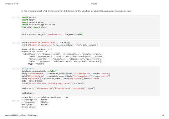
In this programm i will chek the frequency of distribution for the Variables for alcohol consumption, incomeperperson,

```python

import pandas

import numpy

import seaborn as sns

data = pandas.read_csv("gapminder.csv", low_memory=False)

print ("Number of Observations: ", len(data))

print ("Number of Variables: ", len(data.columns))

```

Number of Observations: 213

Number of Variables: 16

```python

print ("Number of Observations: ", len(data))

print ("Number of Variables: ", len(data.columns) ,"\n", data.columns )

```

Number of Observations: 213

Number of Variables: 16

Index(['country', 'incomeperperson', 'alcconsumption', 'armedforcesrate',

'breastcancerper100th', 'co2emissions', 'femaleemployrate', 'hivrate',

'internetuserate', 'lifeexpectancy', 'oilperperson', 'polityscore',

'relectricperperson', 'suicideper100th', 'employrate', 'urbanrate'],

dtype='object')

```python

#clean data

data[data.duplicated(keep=False)]

print("values left after deleting duplicates: ",len(data))

data["alcconsumption"] = pandas.to_numeric(data["alcconsumption"],errors='coerce')

data["lifeexpectancy"] = pandas.to_numeric(data["lifeexpectancy"],errors='coerce')

data["employrate"] = pandas.to_numeric(data["employrate"],errors='coerce')

```

values left after deleting duplicates: 213

Data had no duplicates and is set to numerical so i can start visualizing the frequencies of distribution on my scale

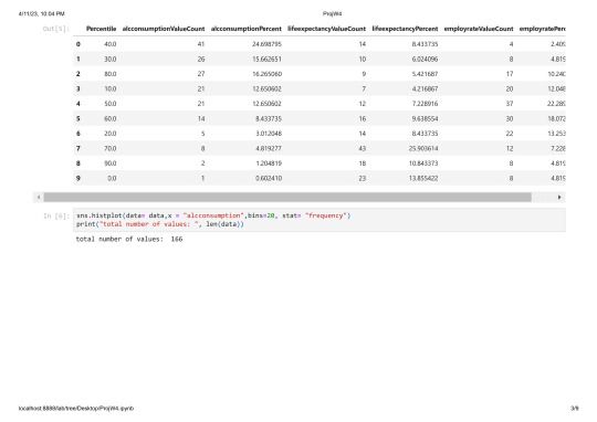
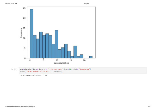
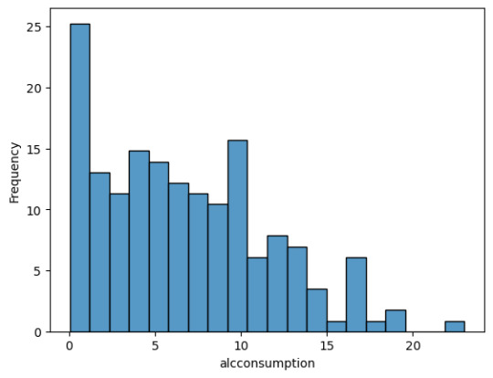
```python

sns.histplot(data= data,x = "alcconsumption",bins=20, stat= "frequency")

print("total number of values: ", len(data))

```

total number of values: 213

![png](output_5_1.png)

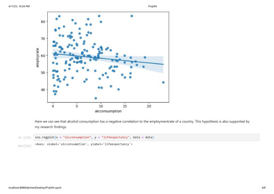
As you can see there are a lot of countries without alcohol consuption and most countries consume arround 1-10 Litres.

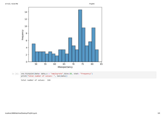
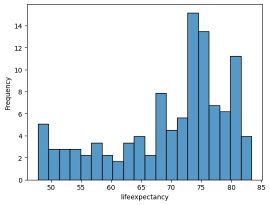
```python

sns.histplot(data= data,x = "lifeexpectancy",bins=20, stat= "frequency")

print("total number of values: ", len(data))

```

total number of values: 213

![png](output_7_1.png)

The lifeexpectancy has a fairly equal distribution wit a peak at around 75 years.

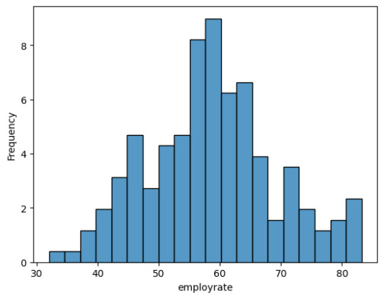
```python

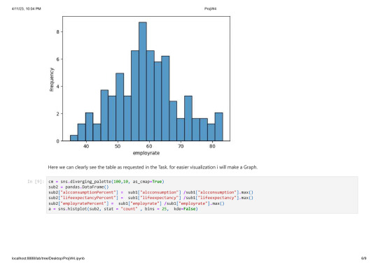
sns.histplot(data= data,x = "employrate",bins=20, stat= "frequency")

print("total number of values: ", len(data))

```

total number of values: 213

![png](output_9_1.png)

The average employment rate is around 60% and ranges from 30 to 80%

0 notes

lukaspyblog · 2 years ago

Text

Peer-graded Assignment: Getting Your Research Project Started

Step1: I want to work with the gapminder Dataset. It has the most interesting data i think. It has so many diffrent interesting datapoints that could be used.

Step2: Research Question: Is alcohol consumption correlated with income, employmentrate and lifeexpectancy?

Hypothesis: I hypothesize that alcohol negativly effects these parameters.

Step3: Codebook

incomeperperson:

2010 Gross Domestic Product per capita in constant 2000 US$. The inflation but not the differences in the cost of living between countries has been taken into account. Scource: World Bank Work Development

alcconsumption:

2008 alcohol consumption per adult (age 15+), litres Recorded and estimated average alcohol consumption, adult (15+) per capita consumption in litres pure alcohol Scource: WHO

employrate:

2007 total employees age 15+ (% of population) Percentage of total population, age above 15, that has been employed during the given year. Scource: International Labour Organization

lifeexpectancy:

2011 life expectancy at birth (years) The average number of years a newborn child would live if current mortality patterns were to stay the same. Scource: 1. Human Mortality Database, 2. World Population Prospects: 3. Publications and files by history prof. James C Riley 4. Human Lifetable Database

urbanrate:

2008 urban population (% of total) Urban population refers to people living in urban areas as defined by national statistical offices (calculated using World Bank population estimates and urban ratios from the United Nations World Urbanization Prospects) Scource: World Bank

Step4: I might check as well if there is an association between all of this and see if there is a correlation between them and urban rate.

Step5: Here is the added Variable needed.

urbanrate:

Step6: Related research. I've looked for: ''alcohol consumption effects society'' , ''alcohol consumption personal wellbeing''

Scource 1

On page 38 it is stated that there is a clear negative effect described that supports my hypothesis.

Scource 2

The summary of this study also cleary correlates a negative impact on societal well being.

Step7: In the study's there is a clear link between alcoholism and it's negative effects on society.

0 notes

lukaspyblog · 2 years ago

Text

Testing the relationship between Tree diameter and sidewalk with roots in stone as a moderator

I got my Dataset from kaggle: https://www.kaggle.com/datasets/yash16jr/tree-census-2015-in-nyc-cleaned

My goal is to check if there is the tree diameter is influenced by it's location on the sidewalk and to use roots in Stone as a moderator variable to check this

```python

import pandas as pd

import statsmodels.formula.api as smf

import seaborn as sb

import matplotlib.pyplot as plt

data = pd.read_csv('tree_census_processed.csv', low_memory=False)

print(data.head(0))

```

Empty DataFrame

Columns: [tree_id, tree_dbh, stump_diam, curb_loc, status, health, spc_latin, steward, guards, sidewalk, problems, root_stone, root_grate, root_other, trunk_wire, trnk_light, trnk_other, brch_light, brch_shoe, brch_other]

Index: []

```python

model1 = smf.ols(formula='tree_dbh ~ C(sidewalk)', data=data).fit()

print (model1.summary())

```

OLS Regression Results

==============================================================================

Dep. Variable: tree_dbh R-squared: 0.063

Model: OLS Adj. R-squared: 0.063

Method: Least Squares F-statistic: 4.634e+04

Date: Mon, 20 Mar 2023 Prob (F-statistic): 0.00

Time: 10:42:07 Log-Likelihood: -2.4289e+06

No. Observations: 683788 AIC: 4.858e+06

Df Residuals: 683786 BIC: 4.858e+06

Df Model: 1

Covariance Type: nonrobust

===========================================================================================

coef std err t P>|t| [0.025 0.975]

-------------------------------------------------------------------------------------------

Intercept 14.8589 0.020 761.558 0.000 14.821 14.897

C(sidewalk)[T.NoDamage] -4.9283 0.023 -215.257 0.000 -4.973 -4.883

==============================================================================

Omnibus: 495815.206 Durbin-Watson: 1.474

Prob(Omnibus): 0.000 Jarque-Bera (JB): 81727828.276

Skew: 2.589 Prob(JB): 0.00

Kurtosis: 56.308 Cond. No. 3.59

==============================================================================

Notes:

[1] Standard Errors assume that the covariance matrix of the errors is correctly specified.

Now i get the data ready to do the moderation variable check after that i check the mean and the standard deviation

```python

sub1 = data[['tree_dbh', 'sidewalk']].dropna()

print(sub1.head(1))

print ("\nmeans for tree_dbh by sidewalk")

mean1= sub1.groupby('sidewalk').mean()

print (mean1)

print ("\nstandard deviation for mean tree_dbh by sidewalk")

st1= sub1.groupby('sidewalk').std()

print (st1)

```

tree_dbh sidewalk

0 3 NoDamage

means for tree_dbh by sidewalk

tree_dbh

sidewalk

Damage 14.858948

NoDamage 9.930601

standard deviation for mean WeightLoss by Diet

tree_dbh

sidewalk

Damage 9.066262

NoDamage 8.193949

To better understand these Numbers I visualize them with a catplot.

```python

sb.catplot(x="sidewalk", y="tree_dbh", data=data, kind="bar", errorbar=None)

plt.xlabel('Sidewalk')

plt.ylabel('Mean of tree dbh')

```

Text(13.819444444444445, 0.5, 'Mean of tree dbh')

![png](output_6_1.png)

its possible to say that there is a diffrence in diameter by the state of the sidewalk now i will check if there is a effect of the roots penetrating stone.

```python

sub2=sub1[(data['root_stone']=='No')]

print ('association between tree_dbh and sidewalk for those whose roots have not penetrated stone')

model2 = smf.ols(formula='tree_dbh ~ C(sidewalk)', data=sub2).fit()

print (model2.summary())

```

association between tree_dbh and sidewalk for those using Cardio exercise

OLS Regression Results

==============================================================================

Dep. Variable: tree_dbh R-squared: 0.024

Model: OLS Adj. R-squared: 0.024

Method: Least Squares F-statistic: 1.323e+04

Date: Mon, 20 Mar 2023 Prob (F-statistic): 0.00

Time: 10:58:36 Log-Likelihood: -1.8976e+06

No. Observations: 543789 AIC: 3.795e+06

Df Residuals: 543787 BIC: 3.795e+06

Df Model: 1

Covariance Type: nonrobust

===========================================================================================

coef std err t P>|t| [0.025 0.975]

-------------------------------------------------------------------------------------------

Intercept 12.3776 0.024 506.657 0.000 12.330 12.426

C(sidewalk)[T.NoDamage] -3.1292 0.027 -115.012 0.000 -3.183 -3.076

==============================================================================

Omnibus: 455223.989 Durbin-Watson: 1.544

Prob(Omnibus): 0.000 Jarque-Bera (JB): 130499322.285

Skew: 3.146 Prob(JB): 0.00

Kurtosis: 78.631 Cond. No. 4.34

==============================================================================

Notes:

[1] Standard Errors assume that the covariance matrix of the errors is correctly specified.

There is still a significant association between them.

Now i check for those whose roots have not penetrated stone.

```python

sub3=sub1[(data['root_stone']=='Yes')]

print ('association between tree_dbh and sidewalk for those whose roots have not penetrated stone')

model3 = smf.ols(formula='tree_dbh ~ C(sidewalk)', data=sub3).fit()

print (model3.summary())

```

association between tree_dbh and sidewalk for those whose roots have not penetrated stone

OLS Regression Results

==============================================================================

Dep. Variable: tree_dbh R-squared: 0.026

Model: OLS Adj. R-squared: 0.026

Method: Least Squares F-statistic: 3744.

Date: Mon, 20 Mar 2023 Prob (F-statistic): 0.00

Time: 11:06:21 Log-Likelihood: -5.0605e+05

No. Observations: 139999 AIC: 1.012e+06

Df Residuals: 139997 BIC: 1.012e+06

Df Model: 1

Covariance Type: nonrobust

===========================================================================================

coef std err t P>|t| [0.025 0.975]

-------------------------------------------------------------------------------------------

Intercept 18.0541 0.031 574.681 0.000 17.993 18.116

C(sidewalk)[T.NoDamage] -2.9820 0.049 -61.186 0.000 -3.078 -2.886

==============================================================================

Omnibus: 72304.550 Durbin-Watson: 1.493

Prob(Omnibus): 0.000 Jarque-Bera (JB): 3838582.479

Skew: 1.739 Prob(JB): 0.00

Kurtosis: 28.416 Cond. No. 2.47

==============================================================================

Notes:

[1] Standard Errors assume that the covariance matrix of the errors is correctly specified.

There is still a significant association between them.

I visualize the means now

```python

print ("means for tree_dbh by sidewalk A vs. B for Roots not in Stone")

m3= sub2.groupby('sidewalk').mean()

print (m3)

sb.catplot(x="sidewalk", y="tree_dbh", data=sub2, kind="bar", errorbar=None)

plt.xlabel('Sidewalk Damage')

plt.ylabel('Tree Diameter at breast height')

```

means for tree_dbh by sidewalk A vs. B for Roots not in Stone

tree_dbh

sidewalk

Damage 12.377623

NoDamage 9.248400

Text(13.819444444444445, 0.5, 'Tree Diameter at breast height')

![png](output_12_2.png)

```python

print ("Means for tree_dbh by sidewalk A vs. B for Roots in Stone")

m4 = sub3.groupby('sidewalk').mean()

print (m4)

sb.catplot(x="sidewalk", y="tree_dbh", data=sub3, kind="bar", errorbar=None)

plt.xlabel('Sidewalk Damage')

plt.ylabel('Tree Diameter at breast height')

```

Means for tree_dbh by sidewalk A vs. B for Roots in Stone

tree_dbh

sidewalk

Damage 18.054102

NoDamage 15.072114

Text(0.5694444444444446, 0.5, 'Tree Diameter at breast height')

![png](output_13_2.png)

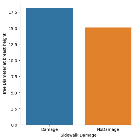
You can definetly see that there is a diffrence in overall diameter as well as its distributions among sidewalk damage an no sidewalk damage.

Therefore you can say that Roots in stone is a good moderator variable and the null hypothesis can be rejected.

0 notes

lukaspyblog · 2 years ago

Text

Generating a Correlation Coefficient

In This analysis i want to check if the opponents rating in a Chess.com Grandmaster match is influenced by the players rating. I got my dataset from Kaggle:

I then import the most important libraries and read my dataset.

```python

import pandas

import seaborn

import scipy

import matplotlib.pyplot as plt

data = pandas.read_csv('chess.csv', low_memory=False)

```

```python

print(data)

```

time_control end_time rated time_class rules \

0 300+1 2021-06-19 11:40:40 True blitz chess

1 300+1 2021-06-19 11:50:06 True blitz chess

2 300+1 2021-06-19 12:01:17 True blitz chess

3 300+1 2021-06-19 12:13:05 True blitz chess

4 300+1 2021-06-19 12:28:54 True blitz chess

... ... ... ... ... ...

859365 60 2021-12-31 16:58:31 True bullet chess

859366 60 2021-04-20 01:12:33 True bullet chess

859367 60 2021-04-20 01:14:49 True bullet chess

859368 60 2021-04-20 01:17:00 True bullet chess

859369 60 2021-04-20 01:19:13 True bullet chess

gm_username white_username white_rating white_result \

0 123lt vaishali2001 2658 win

1 123lt 123lt 2627 win

2 123lt vaishali2001 2641 timeout

3 123lt 123lt 2629 timeout

4 123lt vaishali2001 2657 win

... ... ... ... ...

859365 zuraazmai redblizzard 2673 win

859366 zvonokchess1996 TampaChess 2731 resigned

859367 zvonokchess1996 zvonokchess1996 2892 win

859368 zvonokchess1996 TampaChess 2721 timeout

859369 zvonokchess1996 zvonokchess1996 2906 win

black_username black_rating black_result

0 123lt 2601 resigned

1 vaishali2001 2649 resigned

2 123lt 2649 win

3 vaishali2001 2649 win

4 123lt 2611 resigned

... ... ... ...

859365 ZURAAZMAI 2664 timeout

859366 zvonokchess1996 2884 win

859367 TampaChess 2726 checkmated

859368 zvonokchess1996 2899 win

859369 TampaChess 2717 resigned

[859370 rows x 12 columns]

```python

dup = data[data.duplicated()].shape[0]

print(f"There are {dup} duplicate entries among {data.shape[0]} entries in this dataset.")

#not needed as no duplicates

#data_clean = data.drop_duplicates(keep='first',inplace=True)

#print(f"\nAfter removing duplicate entries there are {data_clean.shape[0]} entries in this dataset.")

```

There are 0 duplicate entries among 859366 entries in this dataset.

Even though the dataset is huge there are no duplicates so i can now check make my plot.

As there are many entires i have to lower the transparency of all points so the Outliers do not affect the overall picture

```python

scat1 = seaborn.regplot(x="white_rating",

y="black_rating",

fit_reg=True, data=data,

scatter_kws={'alpha':0.002})

plt.xlabel('White Rating')

plt.ylabel('Black Rating')

plt.title('Scatterplot for the Association Between the Elo Rate of 2 players')

```

Text(0.5, 1.0, 'Scatterplot for the Association Between the Elo Rate of 2 players')

![png](output_5_1.png)

```python

print ('association between White Rating and Black Rating')

print (scipy.stats.pearsonr(data['white_rating'], data['black_rating']))

```

association between White Rating and Black Rating

PearsonRResult(statistic=0.46087882769619515, pvalue=0.0)

The statistics is fairly high and the P-Value is so low that it actually shows a 0 so we can confidently reject the null hypothesis. We can therefore conclude that there is a statistical relevance between the Player Rating and it's opponent.

The r^2 value is 0.21 therefore we can conclude that 21% of the variablility in the opponents rating can be explained by the Players rating.

0 notes

lukaspyblog · 2 years ago

Text

Peer-graded Assignment: Running a Chi-Square Test of Independence

I got my dataset from Kaggle.

After importing the Modules i first get the Column header to see all

data available

.. code:: ipython3

import pandas as pd

import numpy as np

import scipy.stats as scs

import seaborn as sb

import matplotlib.pyplot as plt

data = pd.read_csv('survey_lung_cancer.csv', low_memory=False)

print(data)

.. parsed-literal::

GENDER AGE SMOKING YELLOW_FINGERS ANXIETY PEER_PRESSURE \

0 M 69 1 2 2 1

1 M 74 2 1 1 1

2 F 59 1 1 1 2

3 M 63 2 2 2 1

4 F 63 1 2 1 1

.. ... ... ... ... ... ...

304 F 56 1 1 1 2

305 M 70 2 1 1 1

306 M 58 2 1 1 1

307 M 67 2 1 2 1

308 M 62 1 1 1 2

CHRONIC DISEASE FATIGUE ALLERGY WHEEZING ALCOHOL CONSUMING \

0 1 2 1 2 2

1 2 2 2 1 1

2 1 2 1 2 1

3 1 1 1 1 2

4 1 1 1 2 1

.. ... ... ... ... ...

304 2 2 1 1 2

305 1 2 2 2 2

306 1 1 2 2 2

307 1 2 2 1 2

308 1 2 2 2 2

COUGHING SHORTNESS OF BREATH SWALLOWING DIFFICULTY CHEST PAIN \

0 2 2 2 2

1 1 2 2 2

2 2 2 1 2

3 1 1 2 2

4 2 2 1 1

.. ... ... ... ...

304 2 2 2 1

305 2 2 1 2

306 2 1 1 2

307 2 2 1 2

308 1 1 2 1

LUNG_CANCER

0 YES

1 YES

2 NO

3 NO

4 NO

.. ...

304 YES

305 YES

306 YES

307 YES

308 YES

[309 rows x 16 columns]

At first i clean from bad column headers the data and remove any

duplicates.

.. code:: ipython3

sub1 = data.rename(columns = {'CHRONIC DISEASE': 'CHRONIC_DISEASE',

'ALCOHOL CONSUMING': 'ALCOHOL_CONSUMING',

'CHEST PAIN' : 'CHEST_PAIN',

'ALLERGY ' : 'ALLERGY',

'SHORTNESS OF BREATH' : 'SHORTNESS_OF_BREATH',

'SWALLOWING DIFFICULTY':'SWALLOWING_DIFFICULTY'})

dup = sub1[sub1.duplicated()].shape[0]

print(f"There are {dup} duplicate entries among {sub1.shape[0]} entries in this dataset.")

sub1.drop_duplicates(keep='first',inplace=True)

print(f"\nAfter removing duplicate entries there are {sub1.shape[0]} entries in this dataset.")

print(sub1.head())

.. parsed-literal::

There are 33 duplicate entries among 309 entries in this dataset.

After removing duplicate entries there are 276 entries in this dataset.

GENDER AGE SMOKING YELLOW_FINGERS ANXIETY PEER_PRESSURE \

0 M 69 1 2 2 1

1 M 74 2 1 1 1

2 F 59 1 1 1 2

3 M 63 2 2 2 1

4 F 63 1 2 1 1

CHRONIC_DISEASE FATIGUE ALLERGY WHEEZING ALCOHOL_CONSUMING COUGHING \

0 1 2 1 2 2 2

1 2 2 2 1 1 1

2 1 2 1 2 1 2

3 1 1 1 1 2 1

4 1 1 1 2 1 2

SHORTNESS_OF_BREATH SWALLOWING_DIFFICULTY CHEST_PAIN LUNG_CANCER

0 2 2 2 YES

1 2 2 2 YES

2 2 1 2 NO

3 1 2 2 NO

4 2 1 1 NO

Now i make a new Dataframe where i check the chi2_contingency pvalue to

see wich parameters my have a significant impact on lung cancer.

.. code:: ipython3

listPval = []

for i in sub1.columns.values.tolist() :

ct = pd.crosstab(sub1[i], sub1['LUNG_CANCER'])

cs = scs.chi2_contingency(ct)

listPval.append(cs.pvalue)

#print('chi-square value and p Value \n',cs)

print(' ',len(listPval), "\n ", len(sub1.columns.tolist()))

pValDict = {'id' : sub1.columns.values.tolist(),

'Pval': listPval}

pValDf = pd.DataFrame(data=pValDict)

print(pValDf)

.. parsed-literal::

id Pval

0 GENDER 4.735015e-01

1 AGE 1.091681e-01

2 SMOKING 6.861518e-01

3 YELLOW_FINGERS 3.013645e-03

4 ANXIETY 2.621869e-02

5 PEER_PRESSURE 2.167243e-03

6 CHRONIC_DISEASE 2.694374e-02

7 FATIGUE 1.333765e-02

8 ALLERGY 8.054292e-08

9 WHEEZING 7.428546e-05

10 ALCOHOL_CONSUMING 2.408699e-06

11 COUGHING 5.652939e-05

12 SHORTNESS_OF_BREATH 3.739728e-01

13 SWALLOWING_DIFFICULTY 1.763519e-05

14 CHEST_PAIN 2.203725e-03

15 LUNG_CANCER 3.706428e-60

Now i visualize said List to make it easier to work with.

.. code:: ipython3

sb.catplot(x='id', y="Pval", data=pValDf, kind="bar", errorbar=None, height=10, aspect = 2.3)

.. parsed-literal::

<seaborn.axisgrid.FacetGrid at 0x179a467cdc0>

.. image:: output_8_1.png

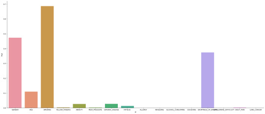
Here we can see that that the most significant statistical correlation

for Lung caner with a p-value of 0.68 is smoking. While Anxiety and

chronic disease show up as well the have a p-value of well below 0.05

wich is not enough to reject the null Hypothesis. Age as an also seems

to have a statistical impact on Lung_caner with a p value of 0.1.

Shortness of breath also has a p-value high enough to reject the null

hypothesis. I would look at gender a bit more closely as it seems

unlikely that gender has an impact on your likelyhood of getting

lungcancer. I check the statistical significance of smoking against

gender to see if one gender somkes more statistically more than the

other.

Here i would do a Post Hoc analysis. My problem is that i don’t know if

the statistical relevance between Lung_cancer and Gender or just between

smoking and Gender. So i check if there is statistical relevance in

smoking and gender.I just check 2 comparisons so i have an adjusted

Post_Hoc pValue of 0.05/2 = 0.025.

.. code:: ipython3

ct = pd.crosstab(sub1['GENDER'], sub1['SMOKING'])

cs = scs.chi2_contingency(ct)

print(ct, '\n',cs)

.. parsed-literal::

SMOKING 1 2

GENDER

F 64 70

M 62 80

Chi2ContingencyResult(statistic=0.316318207753986, pvalue=0.5738287140008982, dof=1, expected_freq=array([[61.17391304, 72.82608696],

[64.82608696, 77.17391304]]))

It’s possible to say that the high P-Value for lung cancer and gender is

caused by the correlation between smoking and gender. Although i can’t

untangle this for certain i’ve shown that the likelyhood for lungcancer

based on Gender seems to be because of diffrent smoking habits.

0 notes

lukaspyblog · 2 years ago

Text

Peer-graded Assignment: Running an analysis of variance

I have chosen to run my Anova and Post hoc in jupyter Notebook and will do my Interpretation in the Markdows. I hope you can excuse my bad grammer and my horrible spelling as i'm not a Native Speaker.

Those are the imported libraries. The dataset is a beginner dataset from kaggle i found(https://www.kaggle.com/datasets/uciml/iris). Feel free to download it if you want to try the Code For yourself.

```python

import numpy as np

import pandas as pd

import statsmodels.formula.api as sm

import statsmodels.stats.multicomp as mlt

data = pd.read_csv('IRIS.csv', low_memory=False)

```

Below i set force my Variables to numeric. Although the Analysis runs just as well without this Step i want to include it as good practice. This is the base Dataset i'm working with

```python

data['sepal-length'] = pd.to_numeric(data['sepal-length'], errors="coerce")

data['sepal-width'] = pd.to_numeric(data['sepal-width'], errors="coerce")

data['petal-length'] = pd.to_numeric(data['petal-length'], errors="coerce")

data['petal-width'] = pd.to_numeric(data['petal-width'], errors="coerce")

print(data)

```

sepal-length sepal-width petal-length petal-width species

0 5.1 3.5 1.4 0.2 Iris-setosa

1 4.9 3.0 1.4 0.2 Iris-setosa

2 4.7 3.2 1.3 0.2 Iris-setosa

3 4.6 3.1 1.5 0.2 Iris-setosa

4 5.0 3.6 1.4 0.2 Iris-setosa

.. ... ... ... ... ...

145 6.7 3.0 5.2 2.3 Iris-virginica

146 6.3 2.5 5.0 1.9 Iris-virginica

147 6.5 3.0 5.2 2.0 Iris-virginica

148 6.2 3.4 5.4 2.3 Iris-virginica

149 5.9 3.0 5.1 1.8 Iris-virginica

[150 rows x 5 columns]

I rename my Column headers because statsmodel doesn't like hyphens when you input it into the formula.

```python

sub1 = data

sub1 = sub1.rename(columns={'sepal-length': 'sepal_length', 'sepal-width': 'sepal_width', 'petal-length' : 'petal_length' , 'petal-width' : 'petal_width'})

print(sub1)

```

sepal_length sepal_width petal_length petal_width species

0 5.1 3.5 1.4 0.2 Iris-setosa

1 4.9 3.0 1.4 0.2 Iris-setosa

2 4.7 3.2 1.3 0.2 Iris-setosa

3 4.6 3.1 1.5 0.2 Iris-setosa

4 5.0 3.6 1.4 0.2 Iris-setosa

.. ... ... ... ... ...

145 6.7 3.0 5.2 2.3 Iris-virginica

146 6.3 2.5 5.0 1.9 Iris-virginica

147 6.5 3.0 5.2 2.0 Iris-virginica

148 6.2 3.4 5.4 2.3 Iris-virginica

149 5.9 3.0 5.1 1.8 Iris-virginica

[150 rows x 5 columns]

In my Anova i want to check if my Petal length is related to the species of the iris. Therefore i drop the other columns and do my OLS.

```python

sub2 = sub1[['petal_length', 'species']].dropna()

model1 = sm.ols(formula='petal_length ~ C(species)', data=sub2)

res1 = model1.fit()

print (res1.summary())

```

OLS Regression Results

==============================================================================

Dep. Variable: petal_length R-squared: 0.941

Model: OLS Adj. R-squared: 0.941

Method: Least Squares F-statistic: 1179.

Date: Wed, 15 Feb 2023 Prob (F-statistic): 3.05e-91

Time: 17:00:24 Log-Likelihood: -84.840

No. Observations: 150 AIC: 175.7

Df Residuals: 147 BIC: 184.7

Df Model: 2

Covariance Type: nonrobust

=================================================================================================

coef std err t P>|t| [0.025 0.975]

-------------------------------------------------------------------------------------------------

Intercept 1.4640 0.061 24.057 0.000 1.344 1.584

C(species)[T.Iris-versicolor] 2.7960 0.086 32.488 0.000 2.626 2.966

C(species)[T.Iris-virginica] 4.0880 0.086 47.500 0.000 3.918 4.258

==============================================================================

Omnibus: 4.393 Durbin-Watson: 2.000

Prob(Omnibus): 0.111 Jarque-Bera (JB): 5.370

Skew: 0.121 Prob(JB): 0.0682

Kurtosis: 3.895 Cond. No. 3.73

==============================================================================

Notes:

[1] Standard Errors assume that the covariance matrix of the errors is correctly specified.

The p Value is very low with only 3.05e-91. This tells me that there is a definite Relationship between petal_length and species. Therefor i reject the Null hypothesis

Now i do a post hoc check to verify wich groups are related to each other.

```python

m2= sub2.groupby('species').mean()

print (m2 ,"\n")

mc1 = mlt.MultiComparison(sub2['petal_length'], sub2['species'])

res1 = mc1.tukeyhsd()

print(res1.summary())

```

petal_length

species

Iris-setosa 1.464

Iris-versicolor 4.260

Iris-virginica 5.552

Multiple Comparison of Means - Tukey HSD, FWER=0.05

===================================================================

group1 group2 meandiff p-adj lower upper reject

-------------------------------------------------------------------

Iris-setosa Iris-versicolor 2.796 0.0 2.5922 2.9998 True

Iris-setosa Iris-virginica 4.088 0.0 3.8842 4.2918 True

Iris-versicolor Iris-virginica 1.292 0.0 1.0882 1.4958 True

-------------------------------------------------------------------

Here you can see that all groups have very diffrent mean Values and we can confidently reject the Null hypothesis

They are all by a significant mean diffrence apart as shown by the reject column.

1 note · View note