machine-learning-for-data-blog

[machine-learning-for-data-blog]

Week 4: K-means Cluster Analysis

A k-means cluster analysis was conducted to identify underlying subgroups of internet user rate based on their similarity of responses on 9 variables that represent characteristics that could have an impact. All clustering variables were standardized to have a mean of 0 and a standard deviation of 1. 

Data were randomly split into a training set that included 70% of the observations and a test set that included 30% of the observations. 

ctrain, ctest = train_test_split(predictors, test_size = 0.3, random_state=123)

A series of k-means cluster analyses were conducted on the training data specifying k=1-9 clusters, using Euclidean distance. 

clusters = range(1,10) mindistance = list()

for val in clusters:    model = KMeans(n_clusters = val)    model.fit(ctrain)    cassign = model.predict(ctrain)    mindistance.append(sum(np.min(cdist(ctrain, model.cluster_centers_, 'euclidean'), axis=1)) / ctrain.shape[0])

The variance in the clustering variables that was accounted for by the clusters (r-square) was plotted for each of the nine cluster solutions in an elbow curve to provide guidance for choosing the number of clusters to interpret. 

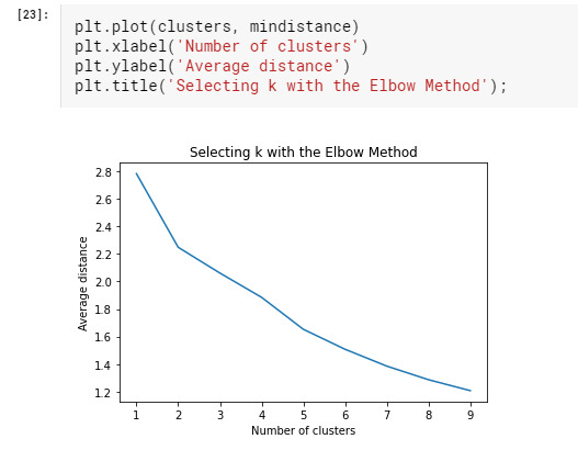
The elbow curve was inconclusive, suggesting that the 2, 4 and 5-cluster solutions might be interpreted. The results below are for an interpretation of the 4-cluster solution.

model3 = KMeans(n_clusters=4) model3.fit(ctrain) cassign = model3.predict(ctrain)

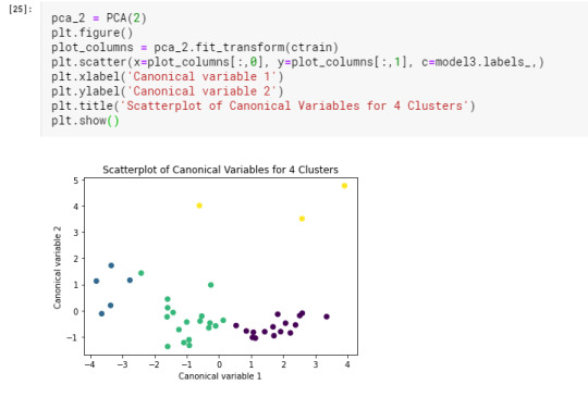
Canonical discriminant analyses was used to reduce the clustering variable down a few variables that accounted for most of the variance in the clustering variables. Observations in cluster one(yellow) were spread out more than the other clusters. internet user rate in cluster zero(green) had the highest clustering variable where cluster three(violet) have moderate variable.

ctrain.reset_index(level=0, inplace=True)

cluslist = list(ctrain['index'])

labels = list(model3.labels_) newlist = dict(zip(cluslist, labels)) print(newlist)

newclus = pd.DataFrame.from_dict(newlist, orient='index') newclus.columns = ['cluster'] newclus.reset_index(level=0, inplace=True) merged_train = pd.merge(ctrain, newclus, on='index') merged_train.head(n=10)

Split internetuserate data into train and test sets 

internetuserate_data = data['internetuserate'] internetuserate_train, internetuserate_test = train_test_split(internetuserate_data, test_size=.3, random_state=123) internetuserate_train1 = pd.DataFrame(internetuserate_train) internetuserate_train1.reset_index(level=0, inplace=True) merged_train_all=pd.merge(internetuserate_train1, merged_train, on='index') sub5 = merged_train_all[['internetuserate', 'cluster']].dropna()

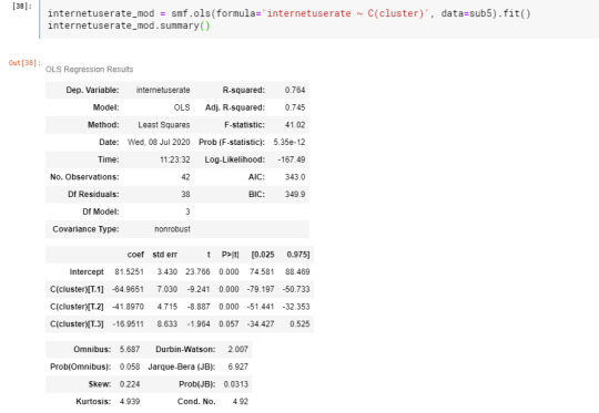
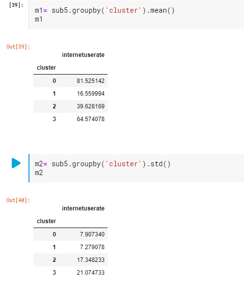
In order to externally validate the clusters, an Analysis of Variance was conducting to test for significant differences between the clusters on grade point average (GPA). Internet user rate in cluster 0 had the highest GPA, and cluster 1 had the lowest GPA. 

[machine-learning-for-data-blog]

Week 3: Lasso Regression

Lasso regression is often used in machine learning to select the subset of variables. The LASSO imposes a constraint on the sum of the absolute values of the model parameters, where the sum has a specified constant as an upper bound. This constraint causes regression coefficients for some variables to shrink towards zero. This model selects only the most important predictors.

features = data[['incomeperperson','employrate','femaleemployrate','polityscore','alcconsumption', 'lifeexpectancy', 'oilperperson','relectricperperson', 'urbanrate']] target = data.internetuserate

predictors = features.copy()

All predictor variables were standardized to have a mean of zero and a standard deviation of one.

predictors['incomeperperson'] = preprocessing.scale(predictors['incomeperperson'].astype('float64')) predictors['employrate'] = preprocessing.scale(predictors['employrate'].astype('float64')) predictors['femaleemployrate'] = preprocessing.scale(predictors['femaleemployrate'].astype('float64')) predictors['polityscore'] = preprocessing.scale(predictors['polityscore'].astype('float64')) predictors['alcconsumption'] = preprocessing.scale(predictors['alcconsumption'].astype('float64')) predictors['lifeexpectancy'] = preprocessing.scale(predictors['lifeexpectancy'].astype('float64')) predictors['oilperperson'] = preprocessing.scale(predictors['oilperperson'].astype('float64')) predictors['relectricperperson'] = preprocessing.scale(predictors['relectricperperson'].astype('float64')) predictors['urbanrate'] = preprocessing.scale(predictors['urbanrate'].astype('float64'))

Data were randomly split into a training set that included 70% of the observations and a test set that included 30% of the observations. 

ftest, ftrain, ttest, ttrain = train_test_split(predictors, target, test_size = 0.3, random_state=123)

The least angle regression algorithm with k=10 fold cross validation was used to estimate the lasso regression model in the training set, and the model was validated using the test set. The change in the cross validation average (mean) squared error at each step was used to identify the best subset of predictor variables.

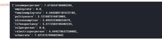
model = LassoLarsCV(cv=10, precompute=False).fit(ftrain, ttrain) dict(zip(predictors.columns, model.coef_))

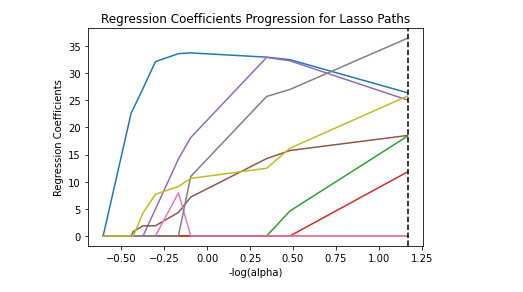
m_log_alphas = -np.log10(model.alphas_) ax = plt.gca() plt.plot(m_log_alphas, model.coef_path_.T) plt.axvline(-np.log10(model.alpha_), linestyle='--', color='k', label='alpha CV') plt.ylabel('Regression Coefficients') plt.xlabel('-log(alpha)') plt.title('Regression Coefficients Progression for Lasso Paths')

Print the r-squared from training and test data

rsquared_train=model.score(pred_train,tar_train) rsquared_test=model.score(pred_test,tar_test) print ('training data R-square') print(rsquared_train) print ('') print ('test data R-square') print(rsquared_test)

So the results show that of the 9 predictor variables, 7 were retained in the selected model. During the estimation process, income per person were most strongly associated with internet user rate, followed by urban rate. These 9 variables accounted for 81% of the variance in the internet user rate response variable.

[machine-learning-for-data-blog]

Week 2: Random Forest

Random forests provide importance scores for each explanatory variable and also allow you to evaluate any increases in correct classification with the growing of smaller and larger number of trees. 

Response Variable: ‘internetuserate’

Explanatory Variables: ‘incomeperperson’, 'employrate’, 'urbanrate’

Importing Required Libraries  

import pandas as pd

from sklearn.model_selection import train_test_split

from sklearn.tree import DecisionTreeClassifier

import sklearn.metrics

from sklearn.ensemble import ExtraTreesClassifier

from sklearn.ensemble import RandomForestClassifier

import numpy as np

import matplotlib.pyplot as plt

%matplotlib inline

Loading Data

data = pd.read_csv(’../input/data-analysis-and-interpretation/_7548339a20b4e1d06571333baf47b8df_gapminder.csv’)

data['internetuserate’] = pd.to_numeric(data['internetuserate’], errors='coerce’) data['incomeperperson’] = pd.to_numeric(data['incomeperperson’], errors='coerce’) data['employrate’] = pd.to_numeric(data['employrate’], errors='coerce’) data['urbanrate’] = pd.to_numeric(data['urbanrate’], errors='coerce’)

Gapminder data set doesn’t contain any binary response variable so conversion is required before performing analysis.

binarydata = data.copy()

def reorder(row):   if row.internetuserate < data.internetuserate.median():       return 0   else:       return 1

binarydata.internetuserate = data.apply(lambda row: reorder(row), axis=1) binarydata.internetuserate.value_counts()

Feature Selection

Here, you need to divide given columns into two types of variables dependent(or target variable) and independent variable(or feature variables).

features = binarydata[['incomeperperson’, 'employrate’, 'urbanrate’]] targets = binarydata.internetuserate

Splitting Data

To understand model performance, dividing the data set into a training set and a test set is a good strategy.

ftrain, ftest, ttrain, ttest = train_test_split(features, targets, test_size=0.4)

Building Model

classifier = RandomForestClassifier(n_estimators=25)

classifier = classifier.fit(features, targets)

prediction = classifier.predict(ftest)

sklearn.metrics.accuracy_score(ttest ,prediction)

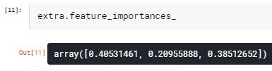
extra = ExtraTreesClassifier() extra.fit(ftrain, ttrain)

Different Number of trees and their effects on accuracy

trees = range(50)

accuracy = np.zeros(50)

for idx in range(len(trees)):   classifier = RandomForestClassifier(n_estimators=idx+1)   classifier = classifier.fit(features, targets)   prediction = classifier.predict(ftest)   accuracy[idx] = sklearn.metrics.accuracy_score(ttest ,prediction)

plt.plot(trees, accuracy) plt.ylabel('Accuracy Score') plt.xlabel('Number of Trees');

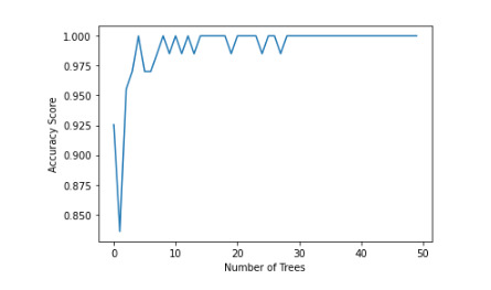
The accuracy of the random forest was 100%, with the subsequent growing of multiple trees rather than a single tree, adding little to the overall accuracy of the model, and suggesting that interpretation of a single decision tree may be appropriate. The training sample has 99 rows and 3 explanatory variable. Testing sample has 67 rows and 3 explanatory variable. Income per person is more associated with internet user rate with 41%. The graph stats that, the accuracy of the model is maintained somehow between 0.975 - 1.

[machine-learning-for-data-blog]

Week 1: Decision Tree

This post is all about decision trees, and more specifically, classification trees. Decision trees are predictive models that allow for a data driven exploration of nonlinear relationships and interactions among many explanatory variables in predicting a response or target variable. When the response variable is categorical (two levels), the model is a called a classification tree. Explanatory variables can be either quantitative, categorical or both. Decision trees create segmentation or subgroups in the data, by applying a series of simple rules or criteria over and over again which choose variable constellations that best predict the response variable.

Response Variable: ‘internetuserate’

Explanatory Variables: 'incomeperperson', 'employrate', 'urbanrate'

Importing Required Libraries  

import pandas as pd from sklearn.model_selection import train_test_split from sklearn.tree import DecisionTreeClassifier import sklearn.metrics

Loading Data

data = pd.read_csv('../input/data-analysis-and-interpretation/_7548339a20b4e1d06571333baf47b8df_gapminder.csv')

data['internetuserate'] = pd.to_numeric(data['internetuserate'], errors='coerce') data['incomeperperson'] = pd.to_numeric(data['incomeperperson'], errors='coerce') data['employrate'] = pd.to_numeric(data['employrate'], errors='coerce') data['urbanrate'] = pd.to_numeric(data['urbanrate'], errors='coerce')

Gapminder data set doesn't contain any binary response variable so conversion is required before performing analysis.

binarydata = data.copy()

def reorder(row):    if row.internetuserate < data.internetuserate.median():        return 0    else:        return 1

binarydata.internetuserate = data.apply(lambda row: reorder(row), axis=1) binarydata.internetuserate.value_counts()

Feature Selection

Here, you need to divide given columns into two types of variables dependent(or target variable) and independent variable(or feature variables).

features = binarydata[['incomeperperson', 'employrate', 'urbanrate']] targets = binarydata.internetuserate

Splitting Data

To understand model performance, dividing the data set into a training set and a test set is a good strategy.

ftrain, ftest, ttrain, ttest = train_test_split(features, targets, test_size=0.4)

Building Decision Tree Model

classifier = DecisionTreeClassifier() classifier = classifier.fit(features, targets)

prediction = classifier.predict(ftest)

Evaluating Model

Let's estimate, how accurately the classifier or model can predict the type of cultivars. Accuracy can be computed by comparing actual test set values and predicted values.

sklearn.metrics.accuracy_score(ttest ,prediction)

Visualizing Decision Trees

In the decision tree chart, each internal node has a decision rule that splits the data.

Decision tree analysis was performed to test nonlinear relationships among a series of explanatory variables and a binary, categorical response variable. All possible separations (categorical) or cut points (quantitative) are tested. For the present analyses, the ‘internet user rate’ is used to grow the tree.

The training sample has 99 rows and 3 explanatory variable. Testing sample has 67 rows and 3 explanatory variable. 

The accuracy score is 1.0, means that the model accurately predicted 100% of the internet use rates per country.