matekon - Tumblr blog

matekon · 5 years ago

Text

What does Galois Theory really tell us?

In the article, I judge the mathematics treated won’t be really developed. Its point will be more of a philosophical nature: to make us think about mathematical abstraction the right way and make us ask the right questions. I know doing so, I risk being a Captain Obvious for some...

I use the following personal conventions:

● - Definitions - Propositions I assume are true

○ - Theorems – Propositions I deduce from the definitions

__________________

We all learned at school the formula for solving quadratic equations.

$ ax^2+bx+c=0$

$\Rightarrow x = \frac{-b \pm \sqrt{b^2-4ac}}{2a} $

Analogous formulas also exist to solve equations of degree 3 and 4, but they are long and painful to use:

Degree 3: https://en.wikipedia.org/wiki/Cubic_equation#Cardano's_formula

Degree 4: https://en.wikipedia.org/wiki/Quartic_function#General_formula_for_roots

For a long time, many mathematicians were searching general formulas for solving equations of degree 5 or more. But then, in the first half of the 19th century, Évariste Galois proved that these formulas just can’t exist. For this, he used some new mathematics he just invented that will later on be called Galois Theory.

You might tell yourself how did he proved such a result. The fact is that I will not talk about Galois Theory directly in this article. I mainly want to be point out that the result above really just is the consequence of a more powerful and surprising result from this theory:

$ \circ $ For any $n \ge 5$, there exists a polynomial of degree $n$ with zeros that aren’t rooty.

Let’s explain the terms.

$ \bullet $ Rooty numbers are the numbers we can construct starting with integers and using the operations of addition, subtraction, multiplication, division and taking roots.

So, examples would be $ \sqrt[3]{2} $ and $\frac{1+\sqrt{5}}{2}$

$ \bullet $ Rooty expressions are all the algebraic expression that we can construct starting with integers and variables and using the operations of addition, subtraction, multiplication, division and taking roots.

Examples would be our 3 formulas above for solving equations of degree 2,3 and 4.

Let’s see the theorem again:

$ \circ $ For any $n \ge 5$, there exists a polynomial of degree $n$ with zeros that aren’t rooty.

Concretely, it is proven that $x^5-x-1$ has no rooty zeros (and is the “simplest” polynomial with this property).

This implies that there isn’t a rooty expression for solving equations of degree 5. That’s because, if there were, when applied to the polynomial $x^5-x-1$, it would return us a rooty number, which would contradict the result just above.

With Galois Theory, we can also find a polynomial of degree 6 with no rooty zeros, implying there isn’t a general formula for solving equations of degree 6. This argument will also work for degrees 7,8,9,... and so on.

That seems shocking as a realization at first, but it really shouldn’t be. I will explain why.

______________________________

Why it shouldn’t be shocking

The fact is that we take operations such as roots as granted, but should we? I would like to point out for instance that you probably haven’t learned a method in school to evaluate it by hand, unlike +,-,* and /.

When we think about it, how are roots defined? There are 2 cases to consider:

First, let’s suppose $n$ odd. Using simple tools from Analysis, we can prove that the polynomial $x^n-a$ must always have one and only one zero in $\mathbb{R}$. So, we define $\sqrt[n]{a}$ as the only real zero of $x^n-a$.

Now, let’s suppose $n$ even. If $a>0$, we can prove that the polynomial $x^n-a$ has exactly 2 zeros on $ \mathbb{R}$, one positive and one negative. So, we can define $\sqrt[n]{a}$ as the positive zero of $x^n-a$ by simple convention. For the case when $a=0$, $x^n-0$ has only $0$ has a zero, so we define $\sqrt[n]{0}=0$. For, $a<0$, $x^n-a$ has no real zeros, so we will decide to not attribute any value to $\sqrt[n]{a}$ in this case.

And that’s pretty much it. I am of the opinion it is more practical to keep the definition of root operations to this and not try to extend it to complex outputs and inputs, mostly because we would lose a lot of nice properties doing so. Consequently, I would not say a thing such as $i = \sqrt{-1} $ for example.

(Ok, I reread the article and realized that the 3 formulas at the beginning do use roots extended to complex numbers and are even used as multivalued functions. Well, conventions go all around the place. But I am sure it is possible to reformulate these formulas using the definition of roots just above.)

Let’s note that, yes, theses definitions are quite “indirect” and don’t allow us to immediately evaluate the values of the roots immediately, but that really shouldn’t be a problem. I prioritize definitions to be intuitive and centered around the comprehension of the concepts. Then, for a function, we should just later on develop ways to evaluate it. We can use Taylor Series or Newton’s method to evaluate roots, among other things.

Roots are “usual’ operations, but that doesn’t make them more “legitimate” than other ones. To illustrate this, let me define a new operation from scratch:

Let’s take $a \in \mathbb{R}$ and $n \in \mathbb{N}$, odd. Then, the polynomial $x^n-x-a$ must absolutely have at least 1 real solution and at most 5 in total. Knowing that, I can define an operation, let’s say $\lhd_n(a)$ which equals the biggest real solution of the polynomial $x^n-x-a$. It will always be well-defined.

Even if it is less frequent as $\sqrt[n]{}$ (well, I just invented it...), $ \lhd_n $ is equally as legitimate, well-defined, computable and all the rest. All I can say against it is that it is probably (definitely!) isn’t as useful of an operation and isn’t as known (obviously...) but that’s about it.

If we want to express all algebraic numbers, using operations such as $ \lhd_n $ would be necessary as roots won’t be enough.

________________________________

Why it should be intuitive

What Galois found is quite intuitive from where I stand and here’s why:

Rooty numbers are what we can build using the structure of very simple polynomials of the form $x^n-a$ and some very basic operations like +,-,* and /.

But polynomials can be a lot more complex than $x^n-a$. So really, expecting every algebraic numbers to be rooty means expecting every polynomial, no matter how complex it is, to have its “internal structure” described by simple polynomials of the form $x^n-a$.

It would be like asking to draw every single shape using only straight lines and circle arcs. Sure, we can make at lot with them, but clearly not everything: it’s way too restrictive.

So, in fact, what’s should be really surprising is that we are able to reduce to $x^n-a$ the polynomials of degrees 2,3 and 4.

___________________________

Some thoughts

You may ask: “Why bother having a rooty formula for solving polynomial equations when I can evaluate the root as precisely as I want using various techniques? What’s the deal with having an exact formula?”.

I don’t think we should see “exact answers” in mathematics as ways to evaluate something. I see it more this way: it is a connection between 2 ideas in math.

For exemple, when Euler proved $\sum_{n=1}^{\infty}\frac{1}{n^2} = \frac{\pi^2}{6}$, he didn’t find a way to evalute the sum. Instead, he found a connection between this summation and circles.

All results in math should better be seeing in this mindframe.

0 notes

matekon · 5 years ago

Text

What do $0^0$ and $0^{-1}$ equal? Undefined vs Indeterminate.

I use the following personal conventions:

● - Definitions - Propositions I assume are true

○ - Theorems – Propositions I deduce from the definitions

Also, just to be clear:

● $ \mathbb{N} = \{0,1,2,3,4…\} $

● $ \mathbb{N}^{*} = \{1,2,3,4...\} $

_____

It is regularly said that $0^0$ is indeterminate, just like it is regularly said that $0$ has no multiplicative inverse $0^{-1}$ (or, equivalently, that we can’t divide by $0$).

But it is important to point out that these 2 cases are very different in nature:

$0^0$ is “indeterminate” and $0^{-1}$ is “undefined”.

This means is the following:

$ \bullet \: $ An expression is indeterminate if it has many possible values.

$ \bullet \: $ An expression is undefined if it has no possible values

Otherwise,

$ \bullet \: $ An expression is well-defined if it has one and only one possible value

(Note: I haven’t taken these definitions out of God’s math book. They are just personal conventions based on my experience. One of my main criteria to evaluate definitions is simply: “Are they useful?”. I am aware that my definition for “indeterminate” could be debated.)

So, $0^{-1}$ being undefined means it has no possible values. We must understand this the following way: giving any value to $0^{-1}$ will necessarily imply a contradiction. It is easy to prove:

Assuming $0^{-1}$ has a value, I can use it in algebraic expressions. Because I defined $0^{-1}$ as the multiplicative inverse of $0$, we immediately get that ...

$ 0*0^{-1}=1 $

$ \Rightarrow 2*(0* 0^{-1}) =2*1$

$ \Rightarrow (2*0)* 0^{-1} =2$

$ \Rightarrow 0*0^{-1} =2$

So, $1=2$ which is a contradiction. So $0^{-1}$ is undefined.

In the other case, $0^0$ is indeterminate because it could either equal $0$ or $1$ and both choices would be totally consistent.

To better understand why this is the case, I really have to start from scratch : I will take the time to define the operation of exponentiation.

First, we all agree that our initial intuitive understanding of exponentiation would be “iterated multiplication”. That’s how we all got introduced to it at school.

Intuitive definition of exponentiation:

$ \bullet \: a^n = a*a*a*...*a$ ($n$ times)

Let’s remark:

1) This definition only makes sense for $ n \in \mathbb{N}^{*} $

2) We see that we can define exponentiation by induction on $n$.

3) Exponentiation is a binary operation. What that means is that it is a function with 2 arguments/inputs.

So with that, let’s make a more rigorous definition for our operation.

Inductive definition of exponentiation with exponent in $ \mathbb{N}^{*}$:

$ \bullet \: exp: \mathbb{C} \times \mathbb{N}^{*} \rightarrow \mathbb{C} $, where $ exp(a,n) = a^n $, is a function so that:

$ (A) \: a^1=a $

$ (B) \: a^{n+1}=a^n*a \: $ for $ n \in \mathbb{N}^{*} $

Let’s remark:

1) Right from the start, we can assume that $a$ can be a complex number. Indeed, this assumption doesn’t create any “problems” with the definition

2) This function is surprisingly uniquely and completely defined without ambiguity by the properties $(A)$ and $(B)$. (How is that?)

What I will do now will seem strange but it’s relevancy will become clear later: I can show that the definition above is logically equivalent to the following:

“Golden” definition of exponentiation with exponent in $ \mathbb{N}^{*}$:

$ \bullet \: exp: \mathbb{C} \times \mathbb{N}^{*} \rightarrow \mathbb{C} $, where $ exp(a,n) = a^n $, is a function so that:

$ (A)\: a^1=a$

$ (B)\: a^{m+n} = a^m*a^n $ for $m,n \in \mathbb{N}^{*} $

I like to think about equation $(B)$ as the “Golden Rule of Exponentiation”: it must ALWAYS be true, regardless of how I want to extend the definition of exponentiation.

As previous, we can show that there is only ONE function that respects the properties $(A)$ and $(B)$.

Our initial goal was to determinate the value for $ 0^0 $. The problem is that our definition above only works for an exponent in $\mathbb{N}^{*} $, which excludes $0$.

So, let’s do what mathematicians love to do : EXTEND the definition above to add $0$ as a possible value for the exponent.

“Golden” definition of exponentiation with exponent in $ \mathbb{N}$:

$ \bullet \: exp: \mathbb{C} \times \mathbb{N} \rightarrow \mathbb{C} $, where $ exp(a,n) = a^n $, is a function so that:

$(1)\: a^1=a $

$ (2)\: a^{m+n} = a^m*a^n $ for $ m,n \in \mathbb{N} $

So, what are the inescapable consequences of this definition? What would happen if the exponent $n$ is $0$?

Case 1: $ a \ne 0 $ and $n=0$

Then, $ a= a^1=a^{1+0}=a^1*a^0 =a*a^0$

$ \Rightarrow a= a*a^0$

$ \Rightarrow 1= a^0$ (by dividing both sides by $a$, which doesn’t equal $0$)

Case 2: $a=0 $ and $n=0$

$0^0 = 0^{0+0}=0^0*0^0$

$ \Rightarrow 0^0 = 0^0*0^0 $

So $0^0$ is a solution of $x=x*x\ \iff x(x-1)=0 $

So $ 0^0 \in \{0,1\} $

And that’s it. Our definition of exponentiation restricts the possible values for $0^0$ to $0$ and $1$. There isn’t enough constraints to impose one specific value.

Unlike the case with $0^{-1}$, we totally could set $0^0=1$ by convention without implying any contradictions and this is often done in practice.

What we just did to define exponentiation can also be done for multiplication.

Multiplication is first introduced as “iterative addition”, so ...

Intuitive definition of exponentiation:

$ \bullet \: a*n = a+a+a+...+a$ ($n$ times)

From that I reformulate it as:

Inductive definition of multiplication with second input in $ \mathbb{N}^{*}$:

$ \bullet \: mult: \mathbb{C} \times \mathbb{N}^{*} \rightarrow \mathbb{C} $, where $ mult(a,n) = a*n $, is a function so that:

$ (A)\: a*1 = a $

$ (B)\: a*(n+1)=a*n+a$ for $n \in \mathbb{N}^{*} $

And I can show that this is equivalent to :

"Golden” definition of multiplication with second input in $ \mathbb{N}^{*}$:

$ \bullet \: mult: \mathbb{C} \times \mathbb{N}^{*} \rightarrow \mathbb{C} $, where $ mult(a,n) = a*n $, is a function so that:

$(A)\: a*1=a $

$(B)\: a*(m+n)=a*m+a*n $ for $m,n \in \mathbb{N}^{*} $

So, the classic rule of distributivity (from the left) would be considered the “Golden Rule of Multiplication” according to my terminology.

</sidenote>

Now I have an important remark to do: There are many definitions for exponentiation, not all of them equivalent. The one I just constructed is the one that is the most directly inferred from our intuitive understanding of exponentiation. But, there is also another quite common definition of this operation, this one using Set Theory:

$ \bullet \: |A|^{|B|} = |\{f:B \rightarrow A\}| $

Surprisingly, with this definition, $0^0$ must equal $1$ and nothing else. (Why?) It is totally well-defined in that case!

So, earlier, when I said $0^0$ is indeterminate, it really is relative to the definition of exponentiation that we choose.

Challenge: How would you extend the “Golden” definition of exponentiation for $ n \in \mathbb{Z}$, then $ n \in \mathbb{Q}$, then $ n \in \mathbb{R}$ and finally $ n \in \mathbb{C}$? You want the properties $(A)$ and $(B)$ to always hold. Would you have to add more properties along the way to make the function well-defined?

0 notes

matekon · 6 years ago

Text

The “best” definition for the sinus and cosinus functions

I use the following personal conventions:

● - Definitions - Propositions I assume are true

○ - Theorems – Propositions I deduce from the definitions

I also prefer $\tau$ which equals $2\pi$ as the circle ratio

_____

In mathematics, there is a common phenomenon: there can be multiple ways of defining the same mathematical object.

For example, here are 2 definitions for an isosceles triangle:

● 1) A triangle is isosceles if it has 2 sides of the same length.

● 2) A triangle is isosceles if it has 2 angles that are equal in measure

These 2 definitions are “equivalent” in the sense that a triangle would be isosceles according to the first definition if and only if it is isosceles according to the second definition. (If you are into analytical philosophy, specifically Frege, you might say these definitions express different “senses” but have the same “reference”.)

The case of the isosceles triangle is pretty simple, but in mathematics, there can be definitions for objects which are equivalent but where it isn’t trivial is the slightest.

Even though it is totally frequent for one mathematical object to have multiple definitions available, the way modern mathematics work (by axiomatisation), we have to choose one definition as a “starting point” and then deduce its equivalence with other definitions later on.

So, with our example of the isosceles triangle, we could either choose the first proposition as our definition and then, the second proposition would follow as a theorem, or we could just as well do the reverse.

But, is there a “starting definition” that is “better” than the others? From experience, I would say that, in the point of view of a “pure mathematician”, this is totally irrelevant and doesn’t matter. But, I do think that we can say some definitions are “better” than others if we allow ourselves to use didactic criteria to evaluate them.

In this article, I will be interested with the functions sinus and cosinus, for which I encountered many different definitions in my school years. In Section 1, I will present these definitions and say what I like and don’t like about them using a didactic approach. Then, in Section 2, I will introduce a definition of these functions that I personally think is the best one and I will show that it is “equivalent” with some of the definitions of Section 1.

__________

Section 1 - The usual definitions for sin and cos

At secondary school, I learned the following definition:

Definition 1 (by the triangle):

$\bullet$ Let $\triangle\ ABC$ be a right triangle where $\angle ABC$ is the right angle

Then we define $sin(\theta)=a/c$ and $cos(\theta)=b/c $.

The pros for this definition are the simplicity of the language and the fact that it is directly applicable to problems of geometry.

Among the cons, we have that this definition only makes senses for $\theta \in ]0,\tau/4[$ (let’s immediately work in radians). Also, I don’t think that this way of presenting sin and cos makes it obvious how to visualize the graphs of these functions. (It is possible to see the graphs but it requires us to be kind of clever.)

You might also say that this definition doesn’t immediately allows us to evaluate the functions for a given input. But I don’t think this is such a big problem and I will explain it soon later.

In CEGEP, I learned the definition involving power series:

Definition 2 (by the power series):

$\bullet \: sin(t) = \sum_{n=0}^{\infty} \frac{(-1)^n}{(2n+1)!}t^{2n+1} = t-\frac{t^3}{3!}+\frac{t^5}{5!}-...$

$ \bullet \:cos(t) = \sum_{n=0}^{\infty} \frac{(-1)^n}{(2n)!}t^{2n} = 1-\frac{t^2}{2!}+\frac{t^4}{4!}-...$

This definition has the main advantage of allowing us to directly calculate the values of the functions. But the inconvenience that immediately comes with these types of definitions is that they make us say: “Where is this coming from? What is its utility?”.

The reality is that I think the human mind prefers to start of with definitions that make us directly see why the object in question is interesting and relevant. And then, for a function, we should find a way to “evaluate” it later on.

Let’s also note that this definition doesn’t make the shape of the graphs any more obvious.

In university, I got introduced to the following definition:

Definition 3 (by the differential equation):

$ \bullet \: sin (t) $ and $cos(t) $ are solutions of the differential equation $ f^{\prime\prime}(t) = -f(t) $

We first note that, because this equation has infinitely many solutions, we need further specifications to precisely define what $sin$ and $cos$ are.

This definition for me just mainly shows us a new interest of the sin and cos functions: there are extremely useful tools for solving differential equations. (This is one of the main motivations behind Fourier Analysis.)

This makes us do an important realization: maybe for didactic reasons, the definition we want to use for different mathematical objects depends on the context: For doing regular problems of geometry, Definition 1 for sin and cos is this best one to use. But for the theory of differential equations, then Definition 3 is more relevant.

I do think this argument is very important. But I also have a weak spot for definitions that are kind of more intuitive, more visual and just more “neutral” and “universal” I would say. I think all these criteria apply to the definition I will introduce in Section 2, which I will call “Definition 4 (by the circle)”. In fact, this definition is quite common, but I have never seen it being formalized the way I am about to do.

____________

Section 2 - The “best” definition for sin and cos

Let’s start with a simple question: “How do I describe a circle?”.

Algebraically, the simplest circle is the one of radius 1 centered at the origin. We define it this way:

$ \bullet \: S^1 = \{ (x,y) \in \mathbb{R}^2 | \: ||(x,y)||=1\} $

We see this way of defining a circle works the following way: We take as points $ (x,y) $ on the circle all the solutions to the equation $ x^2+y^2=1 $.

But what I would like to do instead is to describe the circle with a function, not an equation.

I want a function $f $ that outputs a point on the unit circle given a real number input.

$\bullet\:f:\mathbb{R}\to\mathbb{R}^2$ where $Im(f)=S^1$

We immediately see that $f$ is a vector function (has vectors as outputs). Because of that, it can be separated into 2 scalar functions (have real numbers as outputs).

$ f(t) = (x(t),y(t)) $ where $ x: \mathbb{R} \rightarrow \mathbb{R} $ and $ y: \mathbb{R} \rightarrow \mathbb{R} $

In case you didn’t guessed it, $x(t)$ will become $cos(t)$ and $y(t)$ will become $sin(t)$. I will continue to write them as $x(t)$ and $y(t)$ mainly because this notation makes their role clearer and because they aren’t fully defined yet.

Now, what I want to do is to fully define the functions $x(t)$ and $y(t)$. To do that, I will enumerate a list of properties that I want these 2 functions to have.

Because I said I wanted $f$ to output a point on the unit circle, that implies:

$ f(t) \in S^1 \iff ||f(t)||=1 \iff ||(x(t),y(t))||=1$

$\iff \sqrt{x^2(t)+y^2(t)}=1 \iff x^2(t)+y^2(t)=1 $

With this, I will state the first property to these functions, which is the first part of their Definition 4:

$ \bullet \: (1) \: x^2(t)+y^2(t)=1 $

This property isn’t enough. To illustrate this, let’s remark that the following function $f^{*} $ does obey the property $ (1) $ but isn’t the “nicest” function we could think of:

Basically, we see that $f^{*} $ isn’t “continuous”, because it occasionally “jumps”. But, let’s say I want $f$ to be a function that goes continuously around the circle.

In fact, I want $f $ to be something more specific: “parameterized by arc length”.

This means the following:

● Let $ g(t) $ be a curve in space (2d in this case). Then $ g(t) $ is parameterized by arc length if the length of the arc between $ g(t_0) $ and $g(t_1) $ (where $t_1 > t_0 $ ) is precisely $ t_1 – t_0$.

(In the case of the unit circle, how is this idea related to “radians”?).

I won’t go behind all the theory behind it. It is easy to google anyway. For our purposes, I need to know the theorem that says:

$ \circ \: f $ is “parametrized by arc length” $ \iff ||f’(t)||=1 $

From that I deduce:

$ ||f’(t)||=1 \iff ||(x’(t),y’(t))||=1 $

$\iff (x’(t))^2+(y’(t))^2=1 $

From this, we get the second part of Definition 4:

$ \bullet \: (2) \: (x’(t))^2+(y’(t))^2=1 $

$ f $ being “parameterized by arc length” implies that $ f $ is countinous, as we wanted.

The properties (1) and (2) largely define $ x(t)$ and $y(t)$. In fact, with just these 2 properties, we can show that $ x(t)$ and $y(t)$ must obey Definition 3 (by the differential equation). To prove this is a very fun mathematical exercise. Anyway, here’s my demonstration:

We know:

$ \bullet \: (1) \: x^2+y^2=1 $ $ \bullet \: (2) \: x’^2+y’^2=1 $

We want to show that $ y ^{\prime\prime} =-y $ (The proof for $ x ^{\prime\prime} =-x $ is analogous)

$ (1) \Rightarrow \frac{d}{dt}(x^2+y^2)= \frac{d}{dt}(1) $

$\Rightarrow 2xx’+2yy’=0 $

$\Rightarrow xx’=-yy’$

So, we have: $ \circ \: (A)\: xx’=-yy’\\ $

$ (2) \Rightarrow x^2( x’^2+y’^2)=x^2(1)$

$ \Rightarrow (xx’)^2+(xy’)^2=x^2 $

$\Rightarrow^{(A)} (-yy’)^2+(xy’)^2=x^2 $

$\Rightarrow y’^2(y^2+x^2)=x^2 $

$\Rightarrow^{(1)} y’^2(1)=x^2 \Rightarrow y’^2=x^2 $

Consequently, $ \circ \: (B)\: y’^2=x^2\\ $

$ (B)\Rightarrow \frac{d}{dt}(y’^2)= \frac{d}{dt}(x^2) $

$\Rightarrow 2y’y ^{\prime\prime} =2xx’$

$ \Rightarrow^{(A)} y’y ^{\prime\prime} =-yy’ $

$ \Rightarrow_{*} y ^{\prime\prime} =-y $

(I will call this final equation $ (E_y) $ and use it later)

$QED $

(The last implication with an asterisk below really needs a bit of justification. Because $ y’ $ can equal 0 for some inputs, we can’t just divide by it. But, there is a way to clean up the mess and make the deduction valid.)

As I said before, Definition 3 (by the differential equation) is incomplete in its formulation. So, it’s not because I was able to deduce it from $(1)$ and $(2)$ that these 2 properties are enough to define $ x(t) $ and $ y(t) $.

What I will do now is that I will try do deduce Definition 2 (by the power series). Trying to do so, it will show me what I have to add to $(1)$ and $(2)$ to make the Definition 4 (by the circle) complete.

What I know:

$ (1) \: x^2+y^2=1 $ $ (2) \: x’^2+y’^2=1 $

$ (A)\: xx’=-yy’\\ $ $ (B)\: y’^2=x^2\\ $

$ (E_x) \: x ^{\prime\prime} =-x $ $ (E_y) \: y ^{\prime\prime} =-y $

To deduce Definition 2, I would like to find the Maclaurin Series for $ x(t) $ and $ y(t) $:

$ x(t) = \sum_{n=0}^{\infty} \frac{x^{(n)}(0)}{n!}t^n $

$ y(t) = \sum_{n=0}^{\infty} \frac{y^{(n)}(0)}{n!}t^n $

So, I need to find $ x(0)$, $x’(0)$, $x ^{\prime\prime} (0)$, ... and $y(0)$, $y’(0)$, $y ^{\prime\prime} (0)$,...

$(1)$ and $(2)$ aren’t enough to find the Maclaurin Series. So, I will add the following defining property for $sin$ and $cos$ that is honestly only justifiable as a convention:

$ \bullet \: (3) \: f(0) = (x(0), y(0)) = (1,0) $

So we’ve essentially just chosen the starting point for our curve $ f$. It could just as easily have been $ (0,1)$ or $ (\frac{1}{\sqrt{2}}, \frac{1}{\sqrt{2}} ) $, which also are on the unit circle. This choice for $ f(0) $ is, I think, mainly justifiable as a way to make Definition 4 (by the circle) equivalent to Definition 1 (by the triangle).

Now, let’s use this equation in the quest of finding the Maclaurin Series of $x(t) $ and $ y(t)$ :

From $(3) \: x(0)=1 $ and $ (E_x) \: x ^{\prime\prime} =-x $, I deduce:

$ x^{(4k)}(0)=1 $ and $ x^{(4k+2)}(0)=-1 $ where $k \in \mathbb{N}$

From $ (3) \: y(0)=0 $ and $ (E_y) \: y ^{\prime\prime} =-y $, I deduce:

$ y^{(2k)}(0)=0 $ where $k \in \mathbb{N}$

We are halfway done. But, for the next step, we need to be kind of clever and use an old equation we proved earlier:

$ (B) \: (y’(t))^2= (x(t))^2$

$ \Rightarrow (y’(0)^2=(x(0))^2$

$ \Rightarrow^{(3)} (y’(0))^2=(1)^2 $

$ \Rightarrow y’(0) = \pm 1 $

Again, there is a choice to be made, and again, it is a matter of convention.

It can be shown that choosing $ y’(0)= 1$ will make the vector function $f$ go counterclockwise around the unit circle and that choosing $y’(0)= -1$ will make it go clockwise instead. Yes, we will choose the first option because of the convention of how we measure angles.

$ \bullet \: (4) \: y’(0) = 1 $

This will be the last property we add to Definition 4. Let’s see what we can do with it:

From $ (4) \: y’(0)=1 $ and $ (E_y) \: y ^{\prime\prime} =-y $, I deduce:

$ y^{(4k+1)}(0)=1 $ and $ y^{(4k+3)}(0)=-1 $ where $k \in \mathbb{N}$

From $ (4) \: y’(0)=1 $ and $ (2) \: x’^2+y’^2=1 $, I deduce:

$ (*) \: x’(0) = 0 $

Finally, from $ (*) \: x’(0)=0 $ and $ (E_x) \: x ^{\prime\prime} =-x $, I deduce:

$ x^{(2k+1)}(0)=0 $ where $k \in \mathbb{N}$

Putting all of this together, we finally get the MacLaurin Series:

$ x(t) = \sum_{k=0}^{\infty} \frac{(-1)^{k}}{(2k)!}t^{2k} $

$ y(t) = \sum_{k=0}^{\infty} \frac{(-1)^{k}}{(2k+1)!}t^{2k+1} $

And so we’ve just proven that Definition 4 (we’ve just completed) is equivalent to Definition 2!

For clarity, let’s put all the parts of Definition 4 together and we will posture $x(t) = cos(t) $ and $y(t) = sin(t)$.

Definition 4 (by the circle):

$ \bullet \: sin: \mathbb{R} \rightarrow \mathbb{R} $ and $ cos: \mathbb{R} \rightarrow \mathbb{R} $, where

$ (1)\: cos^2(t)+sin^2(t)=1 $

$ (2)\: (\frac{d}{dt}cos(t))^2+ (\frac{d}{dt}sin(t))^2 =1 $

$ (3)\: sin(0) = 0 $ (which implies $ cos(0) =1) $

$ (4) \: ( \frac{d}{dt}sin(t))|_{t=0} = 1 $

We can also put it on words like that:

Definition 4 (by the circle):

$ \bullet \: f(t) = (cos(t),sin(t)) $ is a function from $\mathbb{R}$ to $\mathbb{R}^2$ where $ Im(f) = S^1$ (unit circle). Also, $ f$ is parameterized by arc length, starts on $ (1,0) $ and goes counterclockwise.

The language can really be seeing as harsh, but once this definition is really understood, it allows us to directly visualize what $sin(t)$ and $cos(t)$ mean. It is also not hard to see the shape of their graphs, especially with the help to the following gif: http://i.imgur.com/jvzRYnC.gif

This is the reason why I think this is the best definition in a didactic point of view.

If we want a more accessible language for people who aren’t specialized in math, this formulation would also be valid:

Definition 4: ● If I start on the unit circle at $ (1,0)$ and I walk t units of distance counterclockwise while staying on the unit circle, my x position will be $cos(t) $ and my y position will be $ sin(t)$

I let to you the proof that Definition 4 is equivalent to Definition 1 (for $ t \in ]0,\tau/4[) $. It is definitely the most straightforward proof on the bunch.

#mathematics #trigonometry #differential equations #calculus

1 note · View note

matekon · 6 years ago

Text

The shortest proof that there are countably many algebraic numbers

This article explores a technique for proving that certain sets are countable that I find so easy, fast and clever that I am surprised it isn’t used more often in casual mathematics. I will present it and then apply it to prove there are countably many algebraic numbers.

I use the following personal conventions:

● - Definitions - Propositions I assume are true

○ - Theorems – Propositions I deduce from the definitions

___________________

Section 0 - Cantor Set Theory (Prerequisites)

I will assume the readers of this article are already a bit familiar with Cantor Set Theory. (If you are not, this video by TED-Ed is a nice accessible introduction: https://www.youtube.com/watch?v=UPA3bwVVzGI)

The point of this section is to fix the definitions really clearly.

$\bullet\:\aleph_0=\vert\mathbb{N}\vert$, meaning Aleph-0 ($\aleph_0$) is defined as the cardinal of the set of the natural numbers ($\mathbb{N}$) $\bullet$ The set A is infinite if $\vert A \vert \ge \aleph_0$ ($\aleph_0$ being the smallest infinity) $\bullet$ The set A is countable if $\vert A \vert \le \aleph_0$

● Given 2 sets $A$ and $B$, $|A| = |B|$(or they have the same cardinality) if I can find a “bijective” function from $A$ to $B$.

From experience, the next 2 definitions are less known from casual mathematicians, but are they crucial for this article.

● Given 2 sets $A$ and $B$ , $|A| \le |B|$ if I can find an “injective” function from $A$ to $B$ .

● Given 2 sets $A$ and $B$ , $|A| \ge |B|$ if I can find a “surjective” function from $A$ to $B$ .

I do realize that these definitions aren’t that trivial. Why they describe our intuitive understanding of “ $|A| \le |B|$ ” and “ $|A| \ge |B|$ ” needs to be thought out a little bit.

Just to illustrate it, let’s take $A= \{a,b,c\}$ and $B = \{d,e,f,g\}$, and then define 2 functions $f$ and $g$ in the following manner:

Because $f$ is injective, that implies that $|A| \le |B|$ or that $3 \le 4$, which is true. Because $g$ is not injective (the “elements” $f$ and g have the same output), its existence does not imply that $|B| \le |A|$ or $4 \le 3$, which would be false.

On the other hand, because $g$ is surjective (all the elements of A are the outputs of some elements of $B$ ), that implies that $|B| \ge |A|$. Similaily, $f$ not being surjective means we can’t deduce that $|A| \ge |B|$.

Finally, we just have to note that we can apply the 3 definitions above ( $|A| = |B|$, $|A| \le |B|$ and $|A| \ge |B|$ ) to infinite sets as well.

___________________

Section 1 - The Technique

We will now present the technique this article is mainly concerned with. Here is its statement:

○ Any set for which all its elements can be expressed in a “finite” sequence using a “finite” alphabet is countable.

To illustrate and clarify this, let’s look at an example:

Let $\mathbb{N}^3$ be the set of all triplets of natural numbers, $(1,3,9)$ being one for example. We easily see that $\mathbb{N}^3$ is infinite. But we would like to show that it is countable. Here’s our plan:

We will conceive a “language” that will allow us to express any triplet possible. For this, we first need the symbols from 0 to 9 to write the natural numbers. Then, we introduce the “:” that will be used to separate the numbers in the triplets. For example, $(1,3,9)$ will be written as “1:3:9″ in this language. So, our alphabet has 11 symbols total!

Now, with this alphabet, I will create the set W, which consists of every finite word that can be written using our alphabet of 11 symbols. “1:3:9″ would be a member of this set, but also words like “2::4::::” which aren’t “grammatical” and don’t represent any triplet.

Here are now the majors lines for our proof:

1) We show that $| \mathbb{N}^3 | \le|W|$. For that, we can create a “surjective” function $ f: W \to \mathbb{N}^3 $ whose existence would imply that $|W|\ge| \mathbb{N}^3|$

2) We show that $|W|\le|\mathbb{N}|$. Again, we just have to construct an “injective” function $g:W\to\mathbb{N}$ and that will imply that $|W|\le|\mathbb{N}|$

And from these 2 inequalities, we deduce that $| \mathbb{N}^3|\le|\mathbb{N}|$

Let’s do the details!

1) I will define a function $ f: W\to \mathbb{N}^3 $ that associates each word of $W$ with its associated triplet if the word is of the form “a:b:c”, where a,b and c are natural numbers. Otherwise, the word would be grammatically incorrect and I will associate the word with the triplet $(0,0,0)$.

For example,

$ f($1:3:9$) = (1,3,9)\in\:\mathbb{N}^3 $

$f($01:03:009$)=(1,3,9)\in \:\mathbb{N}^3 $ (technically a different word from the previous)

$f($2::4::::$) = (0,0,0)\in \: \mathbb{N}^3$ (because it is grammatically incorrect)

We can see that $f$ is surjective because every triplet of $ \mathbb{N}^3 $ is an output of this function. We are done with this part and have shown that $ | \mathbb{N}^3 | \le |W|$.

2) I can define a function $g:W\to\mathbb{N}$ that associates each word of $W$ with a unique natural number by reinterpreting it as a number expressed in base 12. I associate “1″ with $1$, “2″ with $2$, .... “9″ with $9$, “0″ with $10$ and “:” with $11$. I will explain later why I don’t associate “0″ with $0$.

For example,

$g$(1:3:9) $= 1*12^4+11*12^3+3*12^2+11*12^1+9*12^0 \in \mathbb{N}$

$g$(33:0:101)$= 3*12^7+3*12^6+11*12^5+10*12^4+11*12^3+$

$1*12^2+10*12^1+1*12^0 \in \:\mathbb{N}$

You can see that $g$ would never associate 2 different words with the same number, meaning $g$ is injective. That’s because, if we exclude the zeros on the right of the comma and on the left, there is a unique way to write a natural in base 12 (in any natural base bigger than or equal to 2 in general).

So, earlier, I didn’t associate “0″ with $0$ because, otherwise, “3″ and “03″, 2 technically different words, would have the same output by the function $g$, so it wouldn’t be injective.

So, with that, we’ve just proven that $|W| \le | \mathbb{N} | $.

With 1) and 2) together, we deduce:

$\vert \mathbb{N}^3\vert\le\vert\mathbb{N}\vert\Rightarrow | \mathbb{N}^3 |\le\aleph_0\\ $ This really means that $ \mathbb{N}^3$ is “countable”. But we know that $\mathbb{N}^3$ is “infinite”, that is $ | \mathbb{N}^3 |\ge\aleph_0\\ $ So, together, we get that $ \mathbb{N}^3 $ is “countably infinite” or that $ | \mathbb{N}^3 |=\aleph_0\\ $

$QED$

All the great principles behind the technique are there.

The existence of the functions $f$ and $g$ is guaranteed once the condition “every element of our infinite set can be expressed by a finite sequence using a finite alphabet” is verified. So, for now on, when applying this technique, we really don’t have to construct $f$ and $g$ anymore. We can immediately deduce that the set is countable. Thus, the technique gains on speed!

And now…

___________________

Section 2 - The proof that there are countably many algebraic numbers

Let’s make the definition clear:

● All the zeros of polynomials with integer coefficients make up the set of the algebraic numbers.

So, for example, $4/3$ is an algebraic number because it is a (the only) zero of the polynomial $3x-4$. In the same way, $\sqrt[3]{2}$ is algebraic because it’s a zero of $ x^3-2$.

We first note that they are infinitely many algebraic numbers, simply because every natural number is algebraic.

We know:

○ Any set for which all its elements can be expressed in a “finite” sequence using a “finite” alphabet is countable.

So, to prove there are countably many algebraic numbers, we just have to find a finite alphabet that can allow us to express each one of them in a finite sequence.

Expressing every polynomial doesn’t seem like much of a problem. We could just use the numbers from 0 to 9, +, - , ^ and x (14 symbols). For example, the polynomial $ 7x^{12}-10x^5+4 $ is expressed as “7x^12-10x^5+4″.

But, how do we express the zeros of a polynomial?

Trying to express all of them with “rooty expressions” (like $5+\sqrt{3}$) really is too complicated for what we are trying to do. Anyway, we know from Galois Theory that this is impossible in general. There is another, more elegant, way to do it:

It is not hard to show that every polynomial have finitely many zeros. So, I could create a system that can enumerate all of them in a given order. I will decide not to count multiplicity of zeros, so $x^2$ would have just 1 zero.

Let’s take the following zeros of a polynomial in the complex plane:

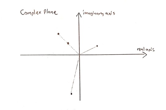
(Yes, this polynomial can’t have real coefficients (why?), but the argument still holds.)

Let’s order them using the following conventions: 1) Zeros are ordered by their arguments (angles) 2) But if 2 zeros have the same argument, then they are ordered by their norms

So, we can order the zeros above like that:

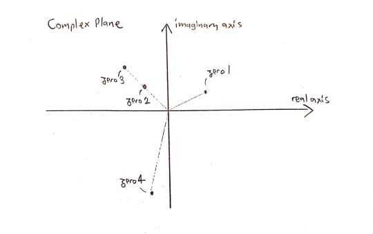
Now, I will introduce “$” in my alphabet. It will work this way:

“ 2$x^5+4x^3-6 ” expresses the 2nd zero of the polynomial $x^5+4x^3-6$.

And … we are done!

We can express every algebraic number with a finite sequence using a finite alphabet of 15 symbols (0, 1, 2, 3, 4, 5, 6, 7, 8, 9, +, -, ^, x and $). It follows from this that there are countably many algebraic numbers.

Also, knowing that there are uncountably many complex numbers, we’ve just proven that transcendental numbers exist (why?).

From experience, I am sure a “pure mathematician” would have written this entire proof in a single paragraph. So, it really is the shortest proof that I know

#mathematics #set theory #numbers

1 note · View note