ml-assignment

[ml-assignment]

Running a Classification Tree

from pandas import Series, DataFrame import pandas as pd import numpy as np import os import matplotlib.pylab as plt from sklearn.model_selection import train_test_split from sklearn.tree import DecisionTreeClassifier from sklearn.metrics import classification_report import sklearn.metrics

os.chdir("C:\TREES")

Load the dataset

AH_data = pd.read_csv("tree_addhealth.csv")

data_clean = AH_data.dropna()

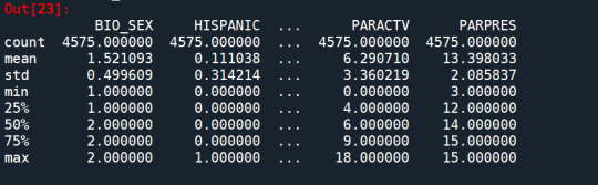
data_clean.dtypes data_clean.describe()

Split into training and testing sets

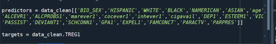
predictors = data_clean[['BIO_SEX','HISPANIC','WHITE','BLACK','NAMERICAN','ASIAN', 'age','ALCEVR1','ALCPROBS1','marever1','cocever1','inhever1','cigavail','DEP1', 'ESTEEM1','VIOL1','PASSIST','DEVIANT1','SCHCONN1','GPA1','EXPEL1','FAMCONCT','PARACTV', 'PARPRES']]

targets = data_clean.TREG1

pred_train, pred_test, tar_train, tar_test = train_test_split(predictors, targets, test_size=.4)

pred_train.shape pred_test.shape tar_train.shape tar_test.shape

Build model on training data

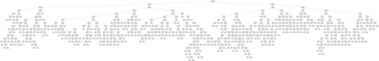
classifier=DecisionTreeClassifier() classifier=classifier.fit(pred_train,tar_train)

predictions=classifier.predict(pred_test)

sklearn.metrics.confusion_matrix(tar_test,predictions) sklearn.metrics.accuracy_score(tar_test, predictions)

Out[28]: 0.7885245901639344

[ml-assignment]

Running a k-means Cluster Analysis

from pandas import Series, DataFrame import pandas as pd import numpy as np import os import matplotlib.pylab as plt

from sklearn.cross_validation import train_test_split

from sklearn.model_selection import train_test_split from sklearn import preprocessing from sklearn.cluster import KMeans

""" Data Management """ os.chdir("C:\TREES") data = pd.read_csv("tree_addhealth.csv")

upper-case all DataFrame column names

data.columns = map(str.upper, data.columns)

Data Management

data_clean = data.dropna()

subset clustering variables

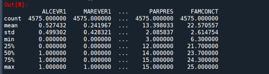
cluster=data_clean[['ALCEVR1','MAREVER1','ALCPROBS1','DEVIANT1','VIOL1', 'DEP1','ESTEEM1','SCHCONN1','PARACTV', 'PARPRES','FAMCONCT']] cluster.describe()

standardize clustering variables to have mean=0 and sd=1

clustervar=cluster.copy() clustervar['ALCEVR1']=preprocessing.scale(clustervar['ALCEVR1'].astype('float64')) clustervar['ALCPROBS1']=preprocessing.scale(clustervar['ALCPROBS1'].astype('float64')) clustervar['MAREVER1']=preprocessing.scale(clustervar['MAREVER1'].astype('float64')) clustervar['DEP1']=preprocessing.scale(clustervar['DEP1'].astype('float64')) clustervar['ESTEEM1']=preprocessing.scale(clustervar['ESTEEM1'].astype('float64')) clustervar['VIOL1']=preprocessing.scale(clustervar['VIOL1'].astype('float64')) clustervar['DEVIANT1']=preprocessing.scale(clustervar['DEVIANT1'].astype('float64')) clustervar['FAMCONCT']=preprocessing.scale(clustervar['FAMCONCT'].astype('float64')) clustervar['SCHCONN1']=preprocessing.scale(clustervar['SCHCONN1'].astype('float64')) clustervar['PARACTV']=preprocessing.scale(clustervar['PARACTV'].astype('float64')) clustervar['PARPRES']=preprocessing.scale(clustervar['PARPRES'].astype('float64'))

split data into train and test sets

clus_train, clus_test = train_test_split(clustervar, test_size=.3, random_state=123)

k-means cluster analysis for 1-9 clusters

from scipy.spatial.distance import cdist clusters=range(1,10) meandist=[]

for k in clusters: model=KMeans(n_clusters=k) model.fit(clus_train) clusassign=model.predict(clus_train) meandist.append(sum(np.min(cdist(clus_train, model.cluster_centers_, 'euclidean'), axis=1)) / clus_train.shape[0])

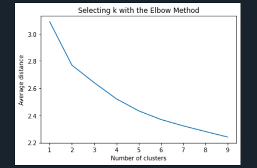
""" Plot average distance from observations from the cluster centroid to use the Elbow Method to identify number of clusters to choose """

plt.plot(clusters, meandist) plt.xlabel('Number of clusters') plt.ylabel('Average distance') plt.title('Selecting k with the Elbow Method')

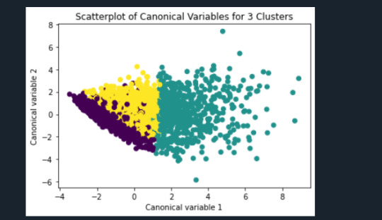
Interpret 3 cluster solution

model3=KMeans(n_clusters=3) model3.fit(clus_train) clusassign=model3.predict(clus_train)

plot clusters

from sklearn.decomposition import PCA pca_2 = PCA(2) plot_columns = pca_2.fit_transform(clus_train) plt.scatter(x=plot_columns[:,0], y=plot_columns[:,1], c=model3.labels_,) plt.xlabel('Canonical variable 1') plt.ylabel('Canonical variable 2') plt.title('Scatterplot of Canonical Variables for 3 Clusters') plt.show()

""" BEGIN multiple steps to merge cluster assignment with clustering variables to examine cluster variable means by cluster """

create a unique identifier variable from the index for the

cluster training data to merge with the cluster assignment variable

clus_train.reset_index(level=0, inplace=True)

create a list that has the new index variable

cluslist=list(clus_train['index'])

create a list of cluster assignments

labels=list(model3.labels_)

combine index variable list with cluster assignment list into a dictionary

newlist=dict(zip(cluslist, labels)) newlist

convert newlist dictionary to a dataframe

newclus=DataFrame.from_dict(newlist, orient='index') newclus

rename the cluster assignment column

newclus.columns = ['cluster']

now do the same for the cluster assignment variable

create a unique identifier variable from the index for the

cluster assignment dataframe

to merge with cluster training data

newclus.reset_index(level=0, inplace=True)

merge the cluster assignment dataframe with the cluster training variable dataframe

by the index variable

merged_train=pd.merge(clus_train, newclus, on='index') merged_train.head(n=100)

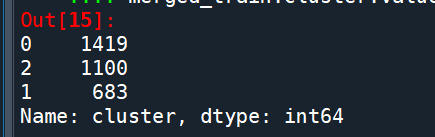
cluster frequencies

merged_train.cluster.value_counts()

""" END multiple steps to merge cluster assignment with clustering variables to examine cluster variable means by cluster """

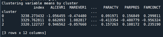
FINALLY calculate clustering variable means by cluster

clustergrp = merged_train.groupby('cluster').mean() print ("Clustering variable means by cluster") print(clustergrp)

validate clusters in training data by examining cluster differences in GPA using ANOVA

first have to merge GPA with clustering variables and cluster assignment data

gpa_data=data_clean['GPA1']

split GPA data into train and test sets

gpa_train, gpa_test = train_test_split(gpa_data, test_size=.3, random_state=123) gpa_train1=pd.DataFrame(gpa_train) gpa_train1.reset_index(level=0, inplace=True) merged_train_all=pd.merge(gpa_train1, merged_train, on='index') sub1 = merged_train_all[['GPA1', 'cluster']].dropna()

import statsmodels.formula.api as smf import statsmodels.stats.multicomp as multi

gpamod = smf.ols(formula='GPA1 ~ C(cluster)', data=sub1).fit() print (gpamod.summary())

print ('means for GPA by cluster') m1= sub1.groupby('cluster').mean() print (m1)

print ('standard deviations for GPA by cluster') m2= sub1.groupby('cluster').std() print (m2)

mc1 = multi.MultiComparison(sub1['GPA1'], sub1['cluster']) res1 = mc1.tukeyhsd() print(res1.summary())

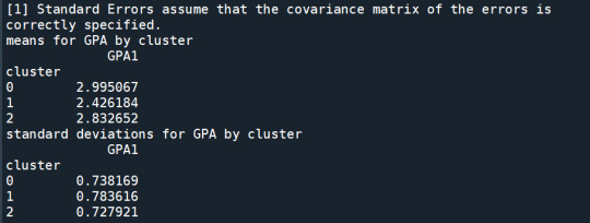
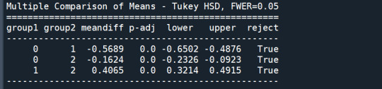
In order to externally validate the clusters, an Analysis of Variance (ANOVA) was conducting to test for significant differences between the clusters on grade point average (GPA). A tukey test was used for post hoc comparisons between the clusters. Results indicated significant differences between the clusters on GPA (F(3, 3197)=82.28, p<.0001). The tukey post hoc comparisons showed significant differences between clusters on GPA, with the exception that clusters 1 and 2 were not significantly different from each other. Adolescents in cluster 4 had the highest GPA (mean=2.99, sd=0.73), and cluster 3 had the lowest GPA (mean=2.42, sd=0.78).

[ml-assignment]

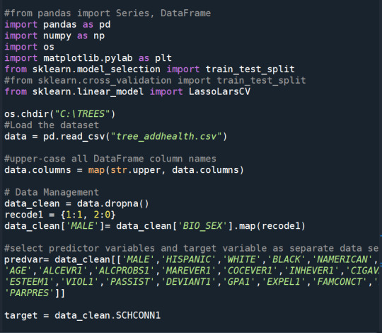
Running a Lasso Regression Analysis

All predictor variables were standardized to have a mean of zero and a standard deviation of one.

Data were randomly split into a training set that included 70% of the observations (N=3201) and a test set that included 30% of the observations (N=1701). The least angle regression algorithm with k=10 fold cross validation was used to estimate the lasso regression model in the training set, and the model was validated using the test set. The change in the cross validation average (mean) squared error at each step was used to identify the best subset of predictor variables.

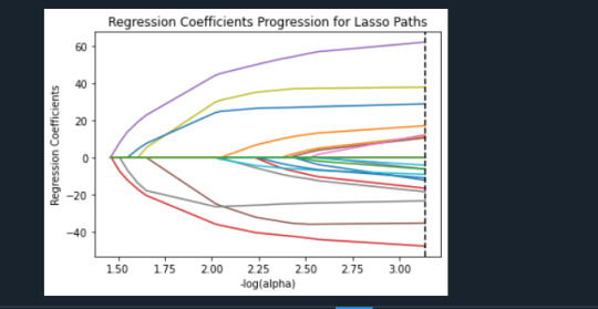
During the estimation process, self-esteem and depression were most strongly associated with school connectedness, followed by engaging in violent behavior and GPA. Depression and violent behavior were negatively associated with school connectedness and self-esteem and GPA were positively associated with school connectedness. Other predictors associated with greater school connectedness included older age, Hispanic and Asian ethnicity, family connectedness, and parental involvement in activities. Other predictors associated with lower school connectedness included being male, Black and Native American ethnicity, alcohol, marijuana, and cocaine use, availability of cigarettes at home, deviant behavior, and history of being expelled from school. These 18 variables accounted for 33.4% of the variance in the school connectedness response variable.

[ml-assignment]

Random Forest

Random forest analysis was performed to evaluate the importance of series of explanatory variables in predicting a binary, categorical response variable. These are the following explanatory variables for evaluating regular smoking.

The explanatory variables with the highest relative importance scores were marijuana (0.12081901) , deviance (0.07145921) and GPA (0.07145921).

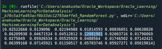
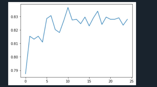
The accuracy of the random forest was 78%, with the subsequent growing of multiple trees rather than a single tree.