panospaterakis

[panospaterakis]

Capstone Project - Week 3

Assignment

[panospaterakis]

Capstone Project - Week 2

Assignment

Methods

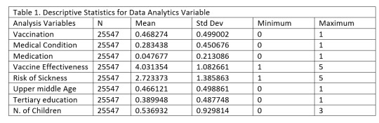
Sample

The sample included N=25547 responders of a random-digit-dialing telephone survey of households about seasonal flu vaccination, designed by the National Center for Health Statistics (NCHS) and the Center for Disease Control and Prevention (CDC). The survey was conducted between October 2009 and June 2010. The individuals answered questions about whether they had received the seasonal flu vaccine, in conjunction with questions about themselves.

Measures

The seasonal vaccination response variable was measured by a binary variable that showed whether the individual received a seasonal flu vaccine or not.

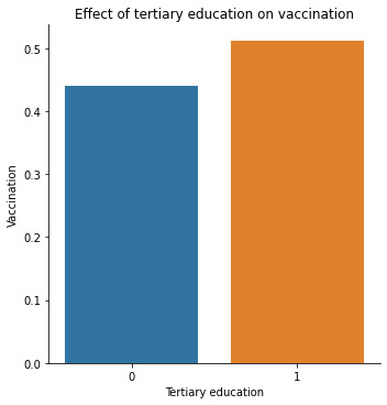
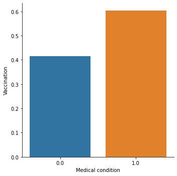
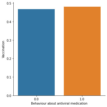
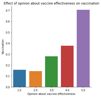
The main predictor of interest is chronic medical condition, a binary variable showing whether the individual has a chronic illness. Other predictors cover social, economic, and demographic background. They include 1) whether the individual has taken antiviral medication (binary), 2) the individual's opinion about seasonal flu vaccine effectiveness (ranging from 1 = Not at all effective to 5 = Very effective), 3) the individual's opinion about the risk of getting sick with seasonal flu without vaccine (ranging from 1 = Not at all effective to 5 = Very effective), 4) being over 55 years old (binary), 5) completed tertiary education (binary) 6) the number of children in household, top-coded to 3.

Analyses

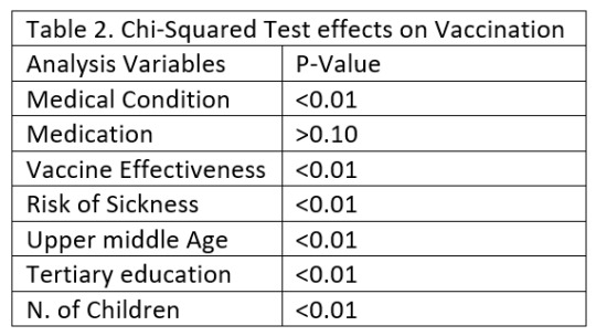
The distributions for the predictors and the seasonal vaccination response variable were evaluated by examining frequency tables for categorical variables and calculating the mean, standard deviation, and minimum and maximum values for quantitative variables.

Bar graphs were also examined, and run chi-squared tests to check the bivariate associations between individual predictors and the seasonal flu vaccination response variable. I used two logistic regression models to find out how chronic illnesses affect the possibility of receiving seasonal vaccination and if this effect moderates when I control for other predictors.

Lasso regression was used to identify the final subset of variables that best predicted the probability of getting the seasonal flu vaccination. The lasso regression model was estimated on a training data set consisting of a random sample of 60% of the responders (N=15328), and a test data set included the other 40% of the responders (N=10219). Before conducting the lasso regression analysis, all predictor variables were standardized to have a mean=0 and standard deviation=1.

[panospaterakis]

Capstone Projest - Week 1

PowerPoint Presentation

Assignment

Research question: Do chronic medical conditions affect the probability of vaccinating against seasonal flu?

 This study aims to identify the effect of chronic medical conditions on the probability of vaccinating against seasonal flu. The response variable is the probability of getting vaccinated against seasonal flu, and the main predictor is chronic illness, while control for other variables like antiviral medication, opinion about vaccine effectiveness, risk of seasonal flu, age group, education, and income.

The Covid 19 era has risen awareness about severe health crises and the importance of vaccination to reduce the victims and the time to reach immunity for the biggest part of the society. As patients with chronic illness are the most vulnerable group to confront severe consequences and are prone to hospitalization from seasonal flu, it is essential to find out if this group is aware of the vaccination, both for their security but also on a national level as previous papers have pointed out the high costs of hospitalization on a federal budget.  

As an economist with an MSc in development economics, I am interested in topics of health and education policies. A possible insignificant effect of chronic illness on the possibility of getting vaccinated would be a sign to apply targeted education policies to grow vaccination awareness, avoid hospitalization, and a possible extensive pressure on the national health system.

[panospaterakis]

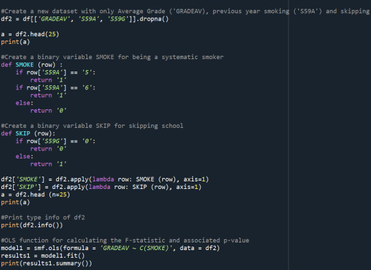
Machine Learning for Data Analysis - Week 4

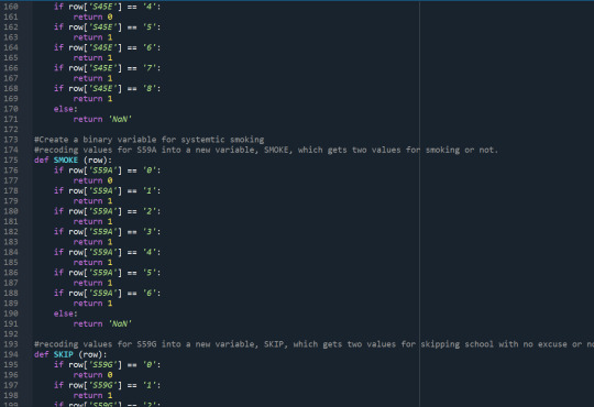
Assignment: Response variable: Excellent average gradeExplanatory variables: Systematic Smoking, Skipping school, Educational aspirations, Gender, White, African American, Asian, American Indian, Parents' education level, Parents' Care, being Adopted You will check the code that I used for this week's assignment below:

Code:

Results:

Summary of the k-means cluster analysis

A k-means cluster analysis was conducted to identify underlying subgroups of adolescents based on their similarity of responses on 11 variables that represent characteristics that could impact school achievement. Clustering variables included The following explanatory variables were included systematic smoking, skipping school, educational aspirations, gender, White, African American, Asian, American Indian, parents' educational level, parents' caring level, and being adopted. All clustering variables were standardized to have a mean of 0 and a standard deviation of 1.

Data were randomly split into a training set that included 70% of the observations (N=990) and a test set that included 30% of the observations (N=425). A series of k-means cluster analyses were conducted on the training data specifying k=1-9 clusters, using Euclidean distance. The variance in the clustering variables that was accounted for by the clusters (r-square) was plotted for each of the nine cluster solutions in an elbow curve to provide guidance for choosing the number of clusters to interpret.

Figure 1. Elbow curve of r-square values for the nine cluster solutions

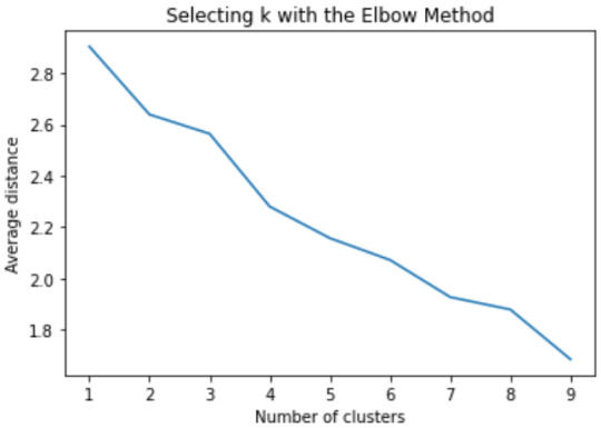
The elbow curve was inconclusive, suggesting that the 2, 3, 4 and 8-cluster solutions might be interpreted. The results below are for an interpretation of the 3-cluster solution.

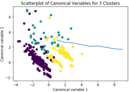
Canonical discriminant analyses was used to reduce the 11 clustering variable down a few variables that accounted for most of the variance in the clustering variables. A scatterplot of the first two canonical variables by cluster (Figure 2 shown below) indicated that the observations in the green cluster, showing high within cluster variance. The other two clusters are densely packed, showing lower within group variance. The three clusters overlap suggesting that maybe it is better to evaluate a two cluster solution.

Figure 2. Plot of the first two canonical variables for the clustering variables by cluster.

The means on the clustering variables showed that, compared to the other clusters, adolescents in cluster 1 had a relatively high likelihood of smoking and skipping school daily and a lower likelihood of having parents that have finished tertiary education. On the other hand, cluster 2 and 3 had approximately the same likelihood of smoking and skipping school daily, while students in cluster 2 have a higher likelihood to have parents with tertiary education.

In order to externally validate the clusters, an Analysis of Variance (ANOVA) was conducted to test for significant differences between the clusters on excellent grade point average (GPA). A tukey test was used for post hoc comparisons between the clusters. Results indicated significant differences between the clusters on excellent GPA (F-stat=11.88, p<0.01). The tukey post hoc comparisons showed significant differences between clusters on excellent GPA, with the exception that clusters 1 and 2 were not significantly different from each other. Students in cluster 3 had the highest chance to receive an excellent average grade (mean=0.42, sd=0.49), and students in cluster 1 had the lowest (mean=0.19, sd=0.39).

[panospaterakis]

Machine Learning for Data Analysis - Week 3

Assignment: Response variable: Excellent average grade

Explanatory variables: Systematic Smoking, Skipping school, Educational aspirations, Gender, White, African American, Asian, American Indian, parents' education level, Parents Care, being adopted 

You will check the code that I used for this week's assignment below:

Code:

Results:

Summary of the LASSO regression:

A lasso regression analysis was conducted to identify a subset of variables from a pool of 11 categorical and quantitative predictor variables that best predicted a quantitative response variable measuring excellent average graduation grade of 4 subjects. The following explanatory variables were included as possible predictors to a Lasso regression evaluating average grade (my response variable), systematic smoking, skipping school, educational aspirations, gender, White, African American, Asian, American Indian, parents' educational level, parents' caring level and being adopted.

Data were randomly split into a training set that included 70% of the observations (N=990) and a test set that included 30% of the observations (N=425). The least angle regression algorithm with k=10 fold cross validation was used to estimate the lasso regression model in the training set, and the model was validated using the test set. The cross-validation average (mean) squared error change at each step was used to identify the best subset of predictor variables.

All of the possible predictors were retained in the selected model. During the estimation process, aspiring to complete tertiary education and be African American were most strongly associated with the chance of graduating with an excellent average grade, followed by being a systematic smoker and having at least a parent who completed tertiary education. Aspiring to complete tertiary education and having at least a parent who completed tertiary education were positively associated with the chance of completing tertiary education with an excellent grade, and being African American and being a systematic smoker were negatively associated with the chance of completing tertiary education. Other predictors associated with a higher chance of having an excellent average grade are being White, Asian, and having parents who care a lot for their children. Other predictors associated with lower chance of having an excellent average grade are being male, being American Indian and being adopted. These 11 variables accounted for 10.7% and 7.6% of the variance of graduating with an excellent average grade for the training and test dataset respectively.

[panospaterakis]

Machine Learning for Data Analysis - Week 2

Assignment:

Response variable: Excellent average grade

Explanatory variables: Systematic Smoking, Skipping school, Educational aspirations, Gender, White, African American, Asian, American Indian, parents' education level, Parents Care, being adopted

 You will check the code that I used for this week's assignment below:

Code:

Results:

Summary of the classification tree

Random forest analysis was performed to evaluate the importance of a series of explanatory variables in predicting a binary response variable. The following explanatory variables were included as possible contributors to a random forest evaluating average grade (my response variable), systematic smoking, skipping school, educational aspirations, gender, White, African American, Asian, American Indian, parents' educational level, parents' caring level and being adopted.

I used a 60% training sample (X_train=849, X=1415) and 40% test sample (X_test=566, X=1415) for the random forest analysis. Using systematic smoking, systematic skipping school, educational aspirations, gender, White, African American, Asian, American Indian, parents' education level, parents' caring level, and being adopted as explanatory variables, the accuracy of the random forest was 63.60%. The explanatory variable with the highest relative importance score was parents' educational level. The subsequent growing of multiple trees rather than a single tree didn't add anything to the model's overall accuracy, suggesting that interpretation of a single decision tree may be appropriate.

[panospaterakis]

Machine Learning for Data Analysis - Week 1

Assignment

Response variable: Excellent average grade

Explanatory variables: Systematic Smoking, Skipping school, Immigration status, parents' education level

 You will check the code that I used for this week's assignment below:

Code:

Results:

Summary of the classification tree

The Decision tree analysis was performed to test nonlinear relationships among a series of explanatory variables and a binary response variable. I used a 60% training sample (X_train=1096, X=1828) and 40% test sample (X_test=732, X=1828) for the classification tree analysis. Using systematic smoking habits, skipping school, immigration status, and parents' educational level as control variables, the decision tree correctly predicts 63.69% of the test sample results.

The parents' educational level (if at least one of the parents received tertiary education) was the variable to separate the sample into two subgroups. Students with at least one parent with tertiary education are more likely to be excellent graduates than students with parents with lower education (43.14% vs. 28.11%).

[panospaterakis]

Regression Modeling in Practice – Week 4

Assignment

Explanatory variable: Systematic Smoking

Response variable: Excellent average grade

Control variables: Age, Gender, Race, Immigration status, parents' education level

Ho: Systematic smoking doesn't affect the probability of graduating with an excellent average grade.

Hα: Systematic smoking affects the probability of graduating with an excellent average grade.

You will check the code that I used for this week's assignment below:

Code:

Results:

Summary of the Logistic regressions

The logistic regression model results without additional control variables show that systematic smoking is significantly associated with receiving an excellent average grade (p<0.05). Systematic smokers have, on average, a lower probability of receiving an excellent average grade (OR=0.29, CI=0.19-0.45, P<0.05)

After adjusting for potential confounding factors (Age, Gender, Race, Immigration status, Parents' Education Level), I found that most of the control variables were significantly correlated with the average grade. The only control variable that was not significantly associated with the average grade was having an Asian (OR=1.62, CI=0.98-2.66, p>0.05) and Native/American Indian background (OR=0.87, CI=0.50-1.49, p>0.05). Being a systematic smoker significantly affects students' chances of being excellent graduates (OR=0.33, CI=0.21-0.52, p<0.05). Moreover, being a Male (OR=0.73, CI=0.59-0.90, p<0.05), Latin (OR=0.33, CI=0.20-0.53, p<0.05), Black (OR=0.37, CI=0.27-0.49, p<0.05), and being older than the mean age of the students (OR=0.86, CI=0.81-0.92, p<0.05) significantly lowers your chances of becoming an excellent graduate, while having at least one parent that has graduated from the university gives you 1.8 times higher chance to become an excellent graduate (OR=1.82, CI=1.47-2.27, p<0.05). After controlling for the confounding factors, I find that systematic smoking significantly lowers a student's probability of becoming an excellent graduate (OR=0.33, CI=0.21-0.52, p<0.05). So, I conclude that after using the possible confounding factors, the effect of systematic smoking on the excellent average grade still exists. So, I reject the H0 hypothesis that the systematic smoking doesn't affect the probability of graduating with an excellent average grade.

[panospaterakis]

Regression Modeling in Practice – Week 3

Assignment

Explanatory variable: Systematic Smoking

Response variable: Average grade

Control variables: Age, Gender, Race, Immigration status, parents' education level

Ho: Systematic smoking doesn't affect the average grade.

Hα: Systematic smoking affects the average grade.

 You will check the code that I used for this week's assignment below:

Code:

Results:

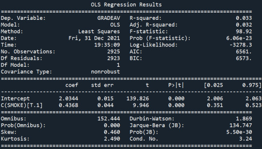
Summary of the OLS regressions

The results of the linear regression model without additional control variables show that systematic smoking (β=0.47, p<0.05) is significantly associated with the average grade (F=64.85, p<0.05). Nonsystematic smokers got, on average, a better grade (Average grade=1.91) than systematic smokers (Average grade=2.38). However, systematic smoking explains only about 3.8% of the data variation (R-squared = 0.038).

After adjusting for potential confounding factors (Age, Gender, Race, Immigration status, Parents' Education Level), I found that most of the control variables were significantly correlated with the average grade (Age_C (β=0.03, r<0.05), Male (β=0.12, r<0.05), Latin (β=0.35, r<0.05, Black (β=0.36, r<0.05), Asian (β=-0.18, r<0.05), Parentsedu (β=-0.22, r<0.05). The only control variable that was not significantly associated with the average grade was Native/American Indian students. Native/American Indian students present a worse average grade relative to White students; however, the p-statistic is greater than 0.05, which may be because of the small sample of Native/ American Indian students (β= 0.08, p> 0.05). After controlling for the confounding factors, I find that systematic smoking still has a stronger effect on average grade than the control variables (β= 0.42, p< 0.05). So, I conclude that after using the possible confounding factors, the effect of systematic smoking on the average grades still exists, rejecting the null hypothesis Η0. The new model with the control variables better predicts the average grade's variability (R-squared= 0.131).  

Q-Q plot

Looking at the diagnostic plots, q-q plot shows that residuals are less normally distributed towards the border quantiles, especially the left lower quantile. This means that the linear regression model may not be a perfect fit for the estimation of the average grade and that I have to consider more variables as control variables.

Standardized residuals for all observations

Plot with standardized residuals for all observations indicates that the majority of the data fits within 1 standard deviation (sd) from the mean. There are fewer observations which fit between 1 and 2 sd, which is fine. Moreover, it seems that about 5% of the values go beyond 2 sd. A few observations go beyond 3 sd, which is a strong indicator of the presence of extreme outliers in my sample, that received extremely low average grade the previous year.

Leverage plot

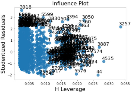
Leverage plot shows, that there are many outliers in the upper left corner with unordinary high values, but small leverage level (0-0.07), which means, they do not strongly influence the estimation of the regression model. There are also a few non-outliers, which significantly influence the estimation of the average grade.

Therefore, we may conclude that the model is a relatively poor fit to our data and including more relevant parameters and/or changing to a non-linear model is needed.

[panospaterakis]

Regression Modeling in Practice – Week 2

Assignment

Explanatory variable: Systematic Smoking

Response variable: Average grade

Ho: Systematic smoking doesn't affect the average grade.

Hα: Systematic smoking affects the average grade.  

You will check the code that I used for this week's assignment below:

Code:

Results:

Summary:

The results of the linear regression model show that systematic smoking (β=0.44, p=0.0001) is significantly associated with the average grade(F=101.1, p<0.0001). Non systematic smokers got on average a better grade (Average grade=2.03), than systematic smokers (Average grade=2.48). However, systematic smoking explains only about 3.3% of the data variation (R-squared = 0.033).

[panospaterakis]

Regression Modeling in Practice – Week 1

Assignment

Sample

The sample is from the first wave of the National Longitudinal Study of Adolescent to Adult Health (AddHealth), a representative school-based survey of adolescents in grades 7-12 in the United States. The first wave focuses on the factors that influence adolescents’ health and risk behaviors, including personal traits, families, friendships, schools, neighborhoods, and communities. The first wave of AddHealth consisted of a sample of 20,745 students in grades 7-12 during the 1994-1995 academic year, who have been followed for five more waves till 2016-2018. AddHealth, in general, gathers through all these waves demographic, socioeconomic, academic, behavioral, psychosocial, cognitive, and health survey data from the initial sampling population and their parents longitudinally. For my analysis, I used all the answers from all the students from the first wave to find if different levels of smoking affect the academic results.

Procedure

AddHealth survey followed a school-based design. 132 middle and high schools were chosen from a stratified by region, urbanicity, school type (public, private, parochial), ethnic mix, and size sample to represent schools from 80 different communities of the USA. The purpose of the data collection was to find the factors that influence adolescents’ health and risk behaviors, including personal traits, families, friendships, schools, neighborhoods, and communities. The first wave of data collection was during the 1994-1995 academic year, while the last wave was in 2016. Data were collected by in-school, in-home, and school administrators’ questionnaires in the first wave of the national longitudinal survey. The wave one in-home sample consisted of 17 randomly chosen students from each stratum, and 100 students from each school, who participated in a 90-minute in-home interview.

Measures

All of the variables of interest have been taken from the in-school questionnaire. The average grade (“At the most recent grading period, what was your grade in each of the following subjects?”) is the average of 4 distinct variables that measure the grade in English/language arts, mathematics, history/social studies, and science. Each categorical variable consists of 4 values representing the grade in each lesson. The smoking level (“During the past 12 months how often did you smoke cigarettes?”) is measured by the frequency of tobacco use the last year that takes seven different values from 0 “Never” to 6 “Nearly everyday”.

[panospaterakis]

Data Analysis Tools – Week 4

Assignment

Explanatory variable: Systematic Smoking

Possible Mediator: Skip school without an excuse

Response variable: Average grade

Ho: Skipping school doesn't moderate the effect of systematic smoking on the average grade.

Hα: Skipping school moderates the effect of systematic smoking on the average grade.

 You will check the code that I used for this week's assignment below:

Code:

Results:

Summary

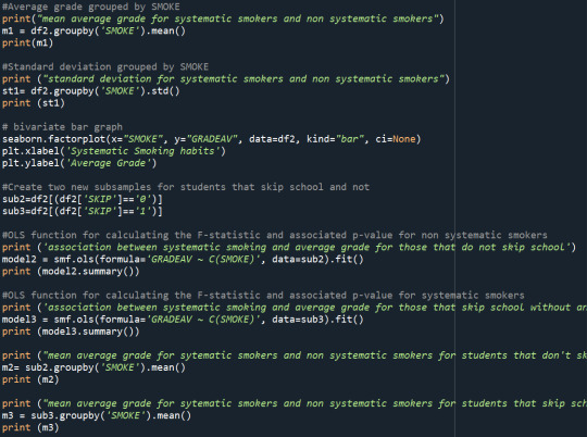
From the above results, I find a significant relationship between systematic smoking and the average grade (p<0.5). On average, systematic smokers received a worse average grade (m=2.47) than the rest of the students (m=2.03). I separated my sample into two groups for students who didn't skip school the previous academic year and ran ANOVA for the two groups separately. I find a significant relationship between systematic smoking and average grade again. In both groups, systematic smokers received worse grades than the rest of the students, while systematic and non-systematic smokers who skipped school the previous year with no excuse received worse grades on average than the same target group that did not skip school the previous year. From the above, I presume that skipping school does not moderate the effect of systematic smoking on the average grade.  

[panospaterakis]

Data Analysis Tools – Week 3

Assignment

Explanatory variable: Level of smoking

Response variable: Average grade

Ho: There isn't any relationship between the level of smoking and the average grade.

Hα: There is a relationship between the level of smoking and average grade.

 You will check the code that I used for this week's assignment below:

Code:

Results:

Summary

With the Pearson correlation, I find a significant relationship between the levels of smoking and the average grade (p<0.5). The scatterplot shows a weak positive linear relationship (r≈0.2) between the levels of smoking and the average grade (as the levels of smoking increase, the average grade also increases). As the highest average grade is 1 and the lowest average grade is 4, this shows that, on average, students that smoke more days per year receive lower grades.

[panospaterakis]

Data Analysis Tools – Week 2

Assignment

Explanatory variable: Level of smoking

Response variable: Excellent average grade

Ho: There is no difference in excellent graduates for each different level of smoking.

Hα: There is a difference in excellent graduates for different levels of smoking.

 You will check the code that I used for this week's assignment below:

Code:

Results

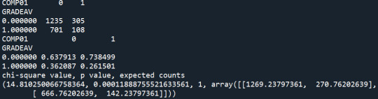
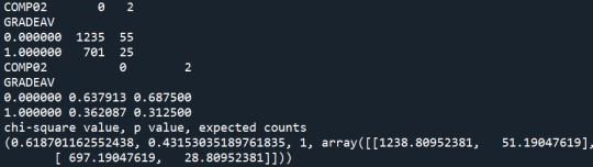
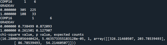
Summary:

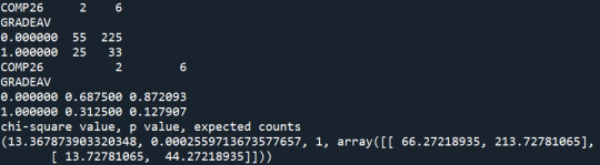
With the Chi-Square test, I find that different levels of smoking affect the probability of students graduating with an excellent average grade (p-value<0.05). The rates of non-smokers graduated with an excellent average grade are the highest, while the rates of daily smokers graduated with an excellent average grade are the lowest. I use the Bonferroni adjustment to check which levels of smoking present significantly different results on the average grade. The levels of smoking are 7 so I need p-value<0.0024 to reject the Ho. The post-hoc tests show that non-smokers (S59A=0) present significantly higher rate of excellent graduates relative to smokers that smoked a few days the previous year (S59A=1), and nearly everyday smokers (S59A>=5).

[panospaterakis]

Data Analysis Tools – Week 1

Assignment Explanatory variable: Level of smoking Response variable: Average grade in English, maths, history, and science Ho: There is no difference in the mean grades of students with different levels of smoking. Hα: There is a difference in the mean grades of students with different levels of smoking.  You will check the code that I used for this week's assignment below: Code:

Results:

Summary:

With the ANOVA, I found that different levels of smoking affect the mean grades of students. The average grades received by non-smokers are the highest, while the average grades received by the everyday smokers are the lowest. The OLS regression shows that the mean differences in students' grades are significantly different based on the levels of smoking (p-value<0.05). The Tukey's HSD test shows that the non-smokers (S59A=0) have different mean grades relative to students that have smoked once or twice the previous year (S59A=1), and students that smoke at least on a weekly basis (S59A>=4), while everyday smokers (S59A=6) get worst mean results relative to students that smoke rarely or non-smokers (S59A<=4).

[panospaterakis]

Data Management and Visualization – Week 4

Assignment

Instructions

Continue with the program you've successfully run.

STEP 1: Create graphs of your variables one at a time (univariate graphs).

Examine both their center and spread.

STEP 2: Create a graph showing the association between your explanatory and response variables (bivariate graph).

Your output should be interpretable (i.e. organized and labeled). 

WHAT TO SUBMIT: 

Once you have written a successful program that creates univariate and bivariate graphs, create a blog entry where you post your program and the graphs that you have created. Write a few sentences describing what your graphs reveal in terms of your individual variables and the relationship between them.

You will check the code that I used for this week's assignment below:

Code:

Visualization - Categorical Variables:

This graph is unimodal with a peak at 2, showing that most of the students received a B in English at the most recent grading period. The graph is skewed to the right, with fewer students receiving a D or lower grades.

This graph is unimodal with a peak at 2, showing that most of the students received a B in Maths at the most recent grading period. The graph is skewed to the right, with fewer students receiving a D or lower grades.

This graph is unimodal with a peak at 8, showing that most of the students are sure that they will graduate from college. The graph is skewed to the left, with fewer students believing that they have low or no chance of finishing tertiary education.

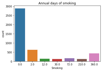
This graph is unimodal with a peak at 0, showing that most of the students are non-smokers. The graph is skewed to the left, with fewer students being smokers.

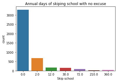
This graph is unimodal with a peak at 0, showing that most of the students didn't skip school in the last 12 months. The graph is skewed to the right, with fewer students skipping school almost every day for the previous 12 months.

Bivariate analysis graphs:

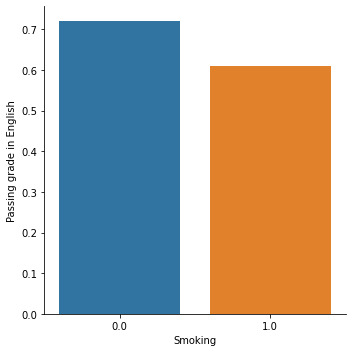
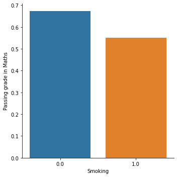
Summary:

With the bivariate analysis, we see that smoking affects educational results. Smokers have a smaller chance of receiving a passing grade in English and Maths, have lower expectations about finishing tertiary education, and skip school more often than non-smokers.

[panospaterakis]

Data Management and Visualization – Week 3

Assignment

Specific rubric items, and their point values, are as follows: Was the program output interpretable (i.e. organized and labeled)? (1 point)

Does the program output display three data managed variables as frequency tables? (1 point)

Did the summary describe the frequency distributions in terms of the values the variables take, how often they take them, the presence of missing data, etc.? (2 points)

You will check the code that I used in Python 3 for this week's assignment below:

Code:

Assignment results (dataset transformation, results of the first 25 rows of the dataset, and frequency distribution of mydataset variables:

Summary:

I recoded the missing values of the variables "S10A", "S10B", "S45E", "S59A", "S59G", such as values that are related to invalid skip and multiple responses to be coded as missing values. Then, I created two new variables, SMOKEPY and SKIPPY, that count for the days of smoking per year and skipped school per year. The frequency results of all the variables can be found above. In general, about 17.78% took A in English, 16.34% took A in Maths, while 32.27% thought they would definitely graduate from college. 44.39% of students haven't smoked the last year, while about 6.53% smoked almost every day. 50.58% of students have never skipped school the previous year, while 0.8% skipped school almost every day.