phoebewang

[phoebewang]

K-Means Cluster Analysis

The code and analysis are below. Please read, thank you!

Figure 1:

Figure 2:

Cluster sizes:

Descriptive Statistics:

Interpretations:

A k-means cluster analysis was conducted to identify subgroups based on patterns in 12 behavioral, demographic, and family-related variables that might be associated with drinking frequency. Clustering variables included demographic indicators such as age and sex, along with several items related to family structure (e.g., FMARITAL, ADULTCH, OTHREL), alcohol-related behaviors (e.g., S1Q7A1, S1Q7A2, S1Q7A3, S1Q7A8, S1Q7A9), and school-related items (e.g., S1Q24LB). Before the analysis, all clustering variables were normalized with a mean of 0 and a standard deviation of 1.

The dataset was randomly split into a training set (70%, N ≈ 29,165) and a test set (30%, N ≈ 12,493). K-means cluster analyses were performed on the training data using Euclidean distance, with solutions ranging from one to nine clusters. In Figure 1, t he average within-cluster distances were shown as an elbow curve. The elbow plot did not provide a clear point of inflection, but it did indicate that a 3-cluster solution may be a viable option for interpretation.

Canonical discriminant analysis was used to reduce the 12 clustering variables to two dimensions for visual purposes as shown in Figure 2. The scatterplot demonstrated that the three groups were slightly distinct in canonical space. Cluster 0 (the purple one) looked to be the biggest group, with more dense organizing, but clusters 1 and 2 (yellow and green) were smaller and more scattered, indicating more within-cluster variability.

Descriptive statistics showed the cluster sizes: Cluster 0 (N=22,998), Cluster 1 (N=5,977), and Cluster 2 (N=1,190). Cluster 1 was characterized by above-average values in S1Q7A1, indicating higher engagement in the “present situation including working full time (35+ hour per week).  and older age. Cluster 2 was differentiated by low values in S1Q7A8 and ADULTCH, suggesting more negative responses related to unemployed and permanently disabled present situation and adult child of respondent in the respondent’s household. Cluster 0 had mean values near the standardized average across most variables.

To externally validate the clusters, an ordinary least squares (OLS) regression was used to determine whether the clusters varied substantially in terms of drinking frequency (DRINKFREQ). The regression results suggested a statistically significant model (F(2, 17071) = 67.66, p < .0001), although the explained variance was modest (R² = 0.008). Post-hoc comparisons showed that Cluster 1 had a substantially greater drinking frequency (b = 0.0855, p <.0001) than Cluster 0, but Cluster 2 had a significantly lower drinking frequency (b = -0.0923, p <.0001). This validates the clusters' discriminant validity in terms of drinking habit.

These results indicates that self-reported drinking frequency varies according to different behavioral and demographic factors. Further investigation of the smallest cluster such as Cluster 2 may reveal protective variables or demographic traits associated with lower alcohol consumption.

Code:

from pandas import Series, DataFrame import pandas as pd import numpy as np import matplotlib.pyplot as plt from sklearn.model_selection import train_test_split from sklearn import preprocessing from sklearn.cluster import KMeans from sklearn.decomposition import PCA from scipy.spatial.distance import cdist import statsmodels.formula.api as smf import statsmodels.stats.multicomp as multi

""""Load dataset""" data = pd.read_csv("_358bd6a81b9045d95c894acf255c696a_nesarc_pds.csv")

""""Uppercase column names""" data.columns = map(str.upper, data.columns)

""""Drop missing values""" data_clean = data.dropna()

""""Subset clustering variables""" cluster = data_clean[['AGE', 'SEX', 'S1Q7A11', 'FMARITAL', 'S1Q7A1', 'S1Q7A8', 'S1Q7A9', 'S1Q7A2', 'S1Q7A3', 'ADULTCH', 'OTHREL', 'S1Q24LB']]

""""tandardize clustering variables""" clustervar = cluster.copy() for col in clustervar.columns: clustervar[col] = preprocessing.scale(clustervar[col].astype('float64'))

""""Split into training and testing sets""" clus_train, clus_test = train_test_split(clustervar, test_size=0.3, random_state=123)

""""K-means clustering with k from 1 to 9 (Elbow method)""" clusters = range(1, 10) meandist = []

for k in clusters: model = KMeans(n_clusters=k, random_state=123) model.fit(clus_train) meandist.append( sum(np.min(cdist(clus_train, model.cluster_centers_, 'euclidean'), axis=1)) / clus_train.shape[0] )

""""Plot Elbow Curve""" plt.figure() plt.plot(clusters, meandist, marker='o') plt.xlabel('Number of Clusters (k)') plt.ylabel('Average Distance to Centroid') plt.title('Elbow Method for Optimal k') plt.grid(True) plt.show()

"""" Fit KMeans for 3 clusters""" model3 = KMeans(n_clusters=3, random_state=123) model3.fit(clus_train) clusassign = model3.predict(clus_train)

""""visualization""" pca_2 = PCA(2) plot_columns = pca_2.fit_transform(clus_train) plt.figure() plt.scatter(x=plot_columns[:, 0], y=plot_columns[:, 1], c=model3.labels_, cmap='viridis') plt.xlabel('Canonical Variable 1') plt.ylabel('Canonical Variable 2') plt.title('Scatterplot of Canonical Variables for 3 Clusters') plt.grid(True) plt.show()

""""Merge cluster assignment with clustering variables""" clus_train.reset_index(level=0, inplace=True) cluslist = list(clus_train['index']) labels = list(model3.labels_) newlist = dict(zip(cluslist, labels)) newclus = DataFrame.from_dict(newlist, orient='index') newclus.columns = ['cluster'] newclus.reset_index(level=0, inplace=True) merged_train = pd.merge(clus_train, newclus, on='index')

""""Cluster frequencies""" print("Cluster sizes:") print(merged_train['cluster'].value_counts())

""""Cluster means""" clustergrp = merged_train.groupby('cluster').mean() print("Clustering variable means by cluster") print(clustergrp)

""""External validation using S2AQ21B - drinking frequency"""

""""Replace blanks and invalid codes"""" data['S2AQ21B'] = data['S2AQ21B'].replace([' ', 98, 99, 'BL'], pd.NA)

""""Drop rows with missing target values"""" data = data.dropna(subset=['S2AQ21B'])

""""Convert to numeric and recode binary target"""" data['S2AQ21B'] = data['S2AQ21B'].astype(int) data['DRINKFREQ'] = data['S2AQ21B'].apply(lambda x: 1 if x in [1, 2, 3, 4] else 0)

drinkfreq_data = data[['DRINKFREQ']] drinkfreq_train, drinkfreq_test = train_test_split(drinkfreq_data, test_size=0.3, random_state=123) drinkfreq_train1 = pd.DataFrame(drinkfreq_train) drinkfreq_train1.reset_index(level=0, inplace=True)

""""Merge with clustering data"""" merged_train_all = pd.merge(drinkfreq_train1, merged_train, on='index') sub1 = merged_train_all[['DRINKFREQ', 'cluster']].dropna()

"""" ANOVA to test cluster differences in DRINKFREQ"""" drinkmod = smf.ols(formula='DRINKFREQ ~ C(cluster)', data=sub1).fit() print(drinkmod.summary())

""""Means and SDs for DRINKFREQ by cluster"""" print('Means for DRINKFREQ by cluster') print(sub1.groupby('cluster').mean())

print('\nStandard deviations for DRINKFREQ by cluster') print(sub1.groupby('cluster').std())

""""Tukey HSD post-hoc test"""" mc1 = multi.MultiComparison(sub1['DRINKFREQ'], sub1['cluster']) res1 = mc1.tukeyhsd() print(res1.summary())

[phoebewang]

LASSO

The dataset was split into training (70%) and testing (30%) subsets.

MSE:

training data MSE=0.17315418324424045 ; test data MSE =0.1702171216510316

R-squared:

training data R-square=0.088021944671551 ; test data R-square = 0.08363901452881095

This graph shows how the mean squared error (MSE) varies with the regularization penalty term (𝛼) during 10-fold cross-validation. Each dotted line indicates the validation error from a single fold, whereas the solid black line is the average MSE over all folds. The vertical dashed line represents the value of 𝛼 that minimized the average MSE, indicating the model's optimal balance of complexity and prediction accuracy.

As 𝛼 decreases (from left to right on the x-axis, as demonstrated by rising −log 10 (α)), the model becomes less regularized, enabling additional predictors to enter. The average MSE initially fell, indicating that adding more variables enhanced the model's performance. However, beyond a certain point, the average MSE smoothed out and slightly rose, indicating possible overfitting when too many predictors were added.

The minimal point on the curve, shown by the vertical dashed line, is the ideal regularization level utilized in the final model. At this phase, the model preserved the subset of variables that had the lowest cross-validated prediction error. The relatively flat tail of the curve indicates that the model's performance was constant throughout a variety of adjacent alpha values, lending confidence to the chosen predictors.

Overall, this graph shows which predictor variables survived after the penalty was applied. Those who survived would have a strong predictive power for the outcome.

This graph shows the coefficient change for each predictor variable in the Lasso regression model based on the regularization penalty term, represented as −log 10(α). As the penalty moves rightward, additional coefficients enter the model and increase in size, demonstrating their importance in predicting drinking frequency.

As shown by the vertical dashed line (alpha CV) representing the optimal alpha level, numerous variables exhibit non-zero coefficients, indicating that they were maintained in the final model as significant predictors of drinking frequency.

The orange and blue line, specifically, suggests a strong prediction pattern of the drinking frequency since they grow rapidly and dominate the model at low regularization levels.

Some other coefficients stay close to 0 or equal to zero across most alpha values, indicating that they were either removed or had few impacts on the final model. The coefficients' stability as regularization lowers indicates that certain predictors have persistent significance regardless of the degree of shrinkage.

Code: A lasso regression analysis was used to determine which factors from a pool of 16 demographic and behavioral predictors best predicted drinking frequency among adult respondents in the NESARC dataset. To ensure that regression coefficients are comparable, all predictors were normalized with a mean of zero and a standard deviation of one. The dataset was divided into training (70%), and testing (30%) sections. The training data was used to apply a lasso regression model with 10-fold cross-validation using Python's LassoCV function. The penalty term (𝛼) was automatically tweaked to reduce cross-validated prediction error.

import pandas as pd import numpy as np import matplotlib.pylab as plt from sklearn.model_selection import train_test_split from sklearn.linear_model import LassoLarsCV

#Load the dataset

data = pd.read_csv("_358bd6a81b9045d95c894acf255c696a_nesarc_pds.csv")

#Data Management

#Subset relevant columns

cols = ['S2AQ21B', 'AGE', 'SEX', 'S1Q7A11', 'FMARITAL','S1Q7A1','S1Q7A8','S1Q7A9','S1Q7A2','S1Q7A3','S1Q1D4','S1Q1D3', 'S1Q1D2','S1Q1D1','ADULTCH','OTHREL','S1Q24LB'] data = data[cols]

#Replace blanks and invalid codes

data['S2AQ21B'] = data['S2AQ21B'].replace([' ', 98, 99, 'BL'], pd.NA)

#Drop rows with missing target values

data = data.dropna(subset=['S2AQ21B'])

#Convert to numeric and recode binary target

data['S2AQ21B'] = data['S2AQ21B'].astype(int) data['DRINKFREQ'] = data['S2AQ21B'].apply(lambda x: 1 if x in [1, 2, 3, 4] else 0)

#select predictor variables and target variable as separate data sets

predvar= data[['AGE', 'SEX', 'S1Q7A11', 'FMARITAL', 'S1Q7A1','S1Q7A8','S1Q7A9','S1Q7A2','S1Q7A3','S1Q1D4','S1Q1D3', 'S1Q1D2','S1Q1D1','ADULTCH','OTHREL','S1Q24LB']]

target = data['DRINKFREQ']

#standardize predictors to have mean=0 and sd=1

predictors=predvar.copy() from sklearn import preprocessing predictors['AGE']=preprocessing.scale(predictors['AGE'].astype('float64')) predictors['SEX']=preprocessing.scale(predictors['SEX'].astype('float64')) predictors['S1Q7A11']=preprocessing.scale(predictors['S1Q7A11'].astype('float64')) predictors['FMARITAL']=preprocessing.scale(predictors['FMARITAL'].astype('float64')) predictors['S1Q7A1']=preprocessing.scale(predictors['S1Q7A1'].astype('float64')) predictors['S1Q7A8']=preprocessing.scale(predictors['S1Q7A8'].astype('float64')) predictors['S1Q7A9']=preprocessing.scale(predictors['S1Q7A9'].astype('float64')) predictors['S1Q7A2']=preprocessing.scale(predictors['S1Q7A2'].astype('float64')) predictors['S1Q7A3']=preprocessing.scale(predictors['S1Q7A3'].astype('float64')) predictors['S1Q1D4']=preprocessing.scale(predictors['S1Q1D4'].astype('float64')) predictors['S1Q1D3']=preprocessing.scale(predictors['S1Q1D3'].astype('float64')) predictors['S1Q1D2']=preprocessing.scale(predictors['S1Q1D2'].astype('float64')) predictors['S1Q1D1']=preprocessing.scale(predictors['S1Q1D1'].astype('float64')) predictors['ADULTCH']=preprocessing.scale(predictors['ADULTCH'].astype('float64')) predictors['OTHREL']=preprocessing.scale(predictors['OTHREL'].astype('float64')) predictors['S1Q24LB']=preprocessing.scale(predictors['S1Q24LB'].astype('float64'))

#split data into train and test sets

pred_train, pred_test, tar_train, tar_test = train_test_split(predictors, target, test_size=.3, random_state=123)

#specify the lasso regression model

from sklearn.linear_model import LassoCV lasso = LassoCV(cv=10, random_state=0).fit(pred_train, tar_train)

#print variable names and regression coefficients

dict(zip(predictors.columns, model.coef_))

--------------

#plot coefficient progression

from sklearn.linear_model import lasso_path

#Compute the full coefficient path

alphas_lasso, coefs_lasso, _ = lasso_path(pred_train, tar_train)

#Plot the coefficient paths

plt.figure(figsize=(10, 6)) neg_log_alphas = -np.log10(alphas_lasso) for coef in coefs_lasso: plt.plot(neg_log_alphas, coef)

plt.axvline(-np.log10(lasso.alpha_), color='k', linestyle='--', label='alpha (CV)') plt.xlabel('-log10(alpha)') plt.ylabel('Coefficients') plt.title('Lasso Paths: Coefficient Progression') plt.legend() plt.tight_layout() plt.show()

-------------------

#plot mean square error for each fold

m_log_alphascv = -np.log10(lasso.alphas_) plt.figure(figsize=(8, 5)) plt.plot(m_log_alphascv, lasso.mse_path_, ':') plt.plot(m_log_alphascv, lasso.mse_path_.mean(axis=-1), 'k', label='Average across the folds', linewidth=2) plt.axvline(-np.log10(lasso.alpha_), linestyle='--', color='k', label='alpha CV') plt.legend() plt.xlabel('-log(alpha)') plt.ylabel('Mean squared error') plt.title('Mean squared error on each fold')

----------------------

#MSE from training and test data

from sklearn.metrics import mean_squared_error train_error = mean_squared_error(tar_train, model.predict(pred_train)) test_error = mean_squared_error(tar_test, model.predict(pred_test)) print ('training data MSE') print(train_error) print ('test data MSE') print(test_error)

----------------------

#R-square from training and test data

rsquared_train=model.score(pred_train,tar_train) rsquared_test=model.score(pred_test,tar_test) print ('training data R-square') print(rsquared_train) print ('test data R-square') print(rsquared_test)

[phoebewang]

Random Forest

This graph shows the accuracy trend of my random forest model as the number of trees increases. The x-axis shows the number of trees, and the y-axis shows the test score. With just a few trees, the model achieves roughly 64% accuracy and rapidly improves. By the time you reach ~5 trees, accuracy exceeds 67%. Increasing the number to 10 to 15, the accuracy stabilizes. Adding more than 15 trees does not improve the performance. Therefore, a small number of trees, up to 15, is the best to get a near-optimal performance. Adding more than 15 has little effect, so it is not necessary. Overall, the graph indicates that no overfitting occurs since accuracy doesn't drop as more trees are added.

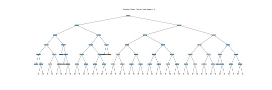
The above tree depicts the Random Forest model's decision trees. Each core node displays a decision rule based on the input variables, whereas the leaf nodes indicate classification results. Due to its depth and complexity, it might not be a good idea for human interpretation, but it does demonstrate how Random Forests incorporate numerous complicated decision boundaries. Here, I show a simplified version of the tree with a depth of 5. This tree alone is unreliable for interpretation, but the forest as a whole makes accurate predictions and emphasizes feature relevance via ensemble learning.

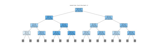
This is a more readable version (depth=3). I will interpret this tree together with a bar graph.

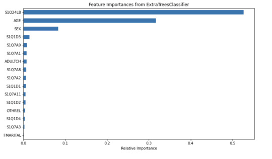
The tree helps visualize the process of classifying a frequent drinker and an infrequent drinker. The root node S1Q24LB(weight) indicates that weight is the most potent variable for splitting the data. Moreover, looking through the bar graph, S1Q24LB has the greatest relative importance. The bar graph confirms that S1Q24LB is the most powerful indicator (shown in the tree), as the model consistently picks them across many trees.

AGE and SEX also appear on the top of the tree, suggesting their importance in decision making. Looking through the bar graph, AGE has the second relative importance. Therefore, it can be concluded that AGE is a strongly predictive factor (but not as important as weight). It indicates that young and old people may have different drinking patterns.

On the other hand, SEX has the thrid relative importance but is much smaller than the AGE. Thus, SEX can be viewed as a moderate predictor. According to the tree, males (SEX=1) are slightly more likely to be classified as frequent drinkers compared to females. SEX is important in decision-making but does not have much separation power. However, it is still important and predictive since it appears in the early split.

Other variables are not that important and predictive.

In conclusion, weight and AGE are two of the most influential predictors in the process of classifying frequent drinkers. While SEX also has its predictive power, it is moderate as compared to weight and AGE. The results shown in the tree can be confirmed by the bar graph of relative importance. Thus, young males with higher weight are more likely to be frequent drinkers.

Code: This is the classifying process.

from pandas import Series, DataFrame import pandas as pd import numpy as np import os import matplotlib.pylab as plt from sklearn.model_selection import train_test_split from sklearn.tree import DecisionTreeClassifier from sklearn.metrics import classification_report import sklearn.metrics # Feature Importance from sklearn import datasets from sklearn.ensemble import ExtraTreesClassifier

#Load the dataset

data = pd.read_csv("_358bd6a81b9045d95c894acf255c696a_nesarc_pds.csv")

#Subset relevant columns

cols = ['S2AQ21B', 'AGE', 'SEX', 'S1Q7A11', 'FMARITAL','S1Q7A1','S1Q7A8','S1Q7A9','S1Q7A2','S1Q7A3','S1Q1D4','S1Q1D3', 'S1Q1D2','S1Q1D1','ADULTCH','OTHREL','S1Q24LB'] data = data[cols]

#Replace blanks and invalid codes

data['S2AQ21B'] = data['S2AQ21B'].replace([' ', 98, 99, 'BL'], pd.NA)

#Drop rows with missing target values

data = data.dropna(subset=['S2AQ21B'])

#Convert to numeric and recode binary target

data['S2AQ21B'] = data['S2AQ21B'].astype(int) data['DRINKFREQ'] = data['S2AQ21B'].apply(lambda x: 1 if x in [1, 2, 3, 4] else 0)

#Define X and y

X = data[['AGE', 'SEX', 'S1Q7A11', 'FMARITAL', 'S1Q7A1','S1Q7A8','S1Q7A9','S1Q7A2','S1Q7A3','S1Q1D4','S1Q1D3', 'S1Q1D2','S1Q1D1','ADULTCH','OTHREL','S1Q24LB']] y = data['DRINKFREQ']

pred_train, pred_test, tar_train, tar_test = train_test_split(X, y, test_size=.4)

pred_train.shape pred_test.shape tar_train.shape tar_test.shape

#Build model on training data

from sklearn.ensemble import RandomForestClassifier

classifier=RandomForestClassifier(n_estimators=25) classifier=classifier.fit(pred_train,tar_train)

predictions=classifier.predict(pred_test)

sklearn.metrics.confusion_matrix(tar_test,predictions) sklearn.metrics.accuracy_score(tar_test, predictions)

#fit an Extra Trees model to the data

model = ExtraTreesClassifier() model.fit(pred_train,tar_train)

#display the relative importance of each attribute

print(model.feature_importances_)

""" Running a different number of trees and see the effect of that on the accuracy of the prediction """

trees=range(25) accuracy=np.zeros(25)

for idx in range(len(trees)): classifier=RandomForestClassifier(n_estimators=idx + 1) classifier=classifier.fit(pred_train,tar_train) predictions=classifier.predict(pred_test) accuracy[idx]=sklearn.metrics.accuracy_score(tar_test, predictions)

plt.cla() plt.plot(trees, accuracy)

Code: Displaying the tree

from sklearn.tree import export_graphviz, plot_tree

#Pick one tree from the forest (e.g., the first one)

estimator = classifier.estimators_[0]

#Plot it using matplotlib

plt.figure(figsize=(30, 10)) plot_tree(classifier.estimators_[0], feature_names=['AGE', 'SEX', 'S1Q7A11', 'FMARITAL', 'S1Q7A1','S1Q7A8','S1Q7A9','S1Q7A2','S1Q7A3','S1Q1D4','S1Q1D3', 'S1Q1D2','S1Q1D1','ADULTCH','OTHREL','S1Q24LB'], class_names=['Not Frequent Drinker', 'Frequent Drinker'], filled=True, rounded=True, max_depth=3) plt.title("Random Forest - Tree #1 (Max Depth = 3)") plt.savefig("random_forest_tree_depth5.png") plt.show()

Code: Creating a bar graph

from sklearn.ensemble import ExtraTreesClassifier

#Train Extra Trees for feature importance

model = ExtraTreesClassifier() model.fit(pred_train, tar_train)

#Create DataFrame for plotting

feat_importances = pd.Series(model.feature_importances_, index=X.columns) feat_importances = feat_importances.sort_values(ascending=True)

#Plot as horizontal bar chart

plt.figure(figsize=(10, 6)) feat_importances.plot(kind='barh') plt.title('Feature Importances from ExtraTreesClassifier') plt.xlabel('Relative Importance') plt.tight_layout() plt.savefig("feature_importance_chart.png") plt.show()

[phoebewang]

Decision Tree Assg#1

Using demographic and behavioral variables, this classification tree predicts whether a person drinks alcohol frequently or infrequently.

The root node splits on SEX, showing that gender is the strongest predictor of drinking frequency.

Those coded as < 1.5 (likely males) are more likely to be frequent drinkers.

Among females, education level (S1Q6A) and age further separated the group, with younger and less educated persons drinking more often.

Other key predictors include:

S1Q1E (origin/descent)

S1Q16 (self-rated health)

AGE

In most branches, frequent drinkers predominate, particularly among younger, less healthy, and male individuals. The tree structure shows how diverse demographic characteristics interact to influence drinking habits.

Code:

import os import pandas as pd import matplotlib.pyplot as plt from sklearn.tree import DecisionTreeClassifier, export_graphviz from sklearn.model_selection import train_test_split from sklearn.metrics import classification_report import graphviz

#Load the data

data = pd.read_csv("_358bd6a81b9045d95c894acf255c696a_nesarc_pds.csv", low_memory=False)

#Subset relevant columns

cols = ['S2AQ21B', 'S1Q1E', 'AGE', 'SEX', 'S1Q1C', 'S1Q16', 'FMARITAL', 'S1Q6A'] data = data[cols]

#Replace blanks and invalid codes

data['S2AQ21B'] = data['S2AQ21B'].replace([' ', 98, 99, 'BL'], pd.NA)

#Drop rows with missing target values

data = data.dropna(subset=['S2AQ21B'])

#Convert to numeric and recode binary target

data['S2AQ21B'] = data['S2AQ21B'].astype(int) data['DRINKFREQ'] = data['S2AQ21B'].apply(lambda x: 1 if x in [1, 2, 3, 4] else 0)

#Define X and y

X = data[['S1Q1E', 'AGE', 'SEX', 'S1Q1C', 'S1Q16', 'FMARITAL', 'S1Q6A']] y = data['DRINKFREQ']

#Train/test split

X_train, X_test, y_train, y_test = train_test_split(X, y, test_size=0.3, random_state=42)

#Train classifier

clf = DecisionTreeClassifier(max_depth=4, random_state=42) clf.fit(X_train, y_train)

#Classification report

print("\nClassification Report:\n") print(classification_report(y_test, clf.predict(X_test)))

#Generate Graphviz output

dot_data = export_graphviz( clf, out_file=None, feature_names=X.columns, class_names=["Infrequent", "Frequent"], filled=False, rounded=True, special_characters=True )

#Render and save the tree as PNG

graph = graphviz.Source(dot_data) graph.render("drink_freq_tree", format="png", cleanup=True) graph.view()