pkreilly

[pkreilly]

Sandbagged

Did we fall for the largest sandbagged quarter ever?

Intro

On March 8th I sent out series of tweets, https://twitter.com/PeterKReilly/status/1104520804824428544,  musing about the sudden drop off in reported operating 4th quarter 2018 earnings margins, basically out of the blue.  This really left me perplexed as to what happened as it was unusual relative to normal developments in corporate earnings. This blog post is a follow up now that we have some more clarity on the trajectory of margins through 1Q 2019 with the intent to lay out the logic and the evidence that yes indeed we were had and that this has distorted the markets view of actual earnings power of publicly traded companies.

The issue

When the dust settled on 4thQ 2018 earnings it became clear that something very unusual happened, out of the blue earnings per share and reported margins broke down.

 Bears seized on this as evidence, along with other weakness in international and domestic economic statistics, that we were in a recession NOW.  What was unusual was that 4Q earnings didn’t increase from the 3rd quarter as is typical due to revenue seasonality and in fact operating margins dropped precipitously from 3rd quarter, which is a strong precursor to secular bear markets.  Markets, in part, reacted to this development of weak guidance and downward earnings revisions and duly sold off hard starting from very stretched valuations in October.  The S&P 500 registered a nearly 20% decline in under 3 months.

The theory

Jonathan Robinson, a fellow participant in Twitter finance discussions @Robohogs, and I developed an alternate explanation, that would be far less negative for future equity prices, but to some would seem outlandish and certainly would need to see some strong evidence to confirm.  The theory goes like this:

1. The timing of the passage of the Tax Cut and Jobs act of 2017, passed by the house only on December 20th and going into effect January 1, 2018 created a very unusual set of incentives for corporations and their leadership and finance professionals that COULD lead to a desire to understate reported earnings in the 4th quarter of 2018.  For details on the timing of passage click the link. 

https://en.wikipedia.org/wiki/Tax_Cuts_and_Jobs_Act_of_2017

2. By the time the tax cut was enacted companies had by then long locked down their financial plans, without any tax benefit as you can’t count on speculation as to its passage in financial plans and guidance, had them approved by their boards and had them built into incentive comp (bonus and other equity comp programs) plans for the companies executives.  The tax cut represented a massive windfall to these programs.  Note that Wall Street sell side analysts massively missed the effect of the tax act in their 2018 estimates as companies did not build it into their guidance. 

3. Long Term comp programs (LTC), used by companies to reward executives for financial performance among other items, typically have protections in their structure to cap payouts so that management does not benefit from windfalls outside the control of management.  The tax cuts were the mother of all windfalls and management stood to benefit from this, up to a point.

4. The cap to LTC programs upside created the incentive for companies to report conservatively in the 4thQ as many bonus and LTC programs would have already capped out at the maximum payout and management would not benefit from the addition earnings in 2018.  The incentive would be to carry earnings over into 2019 to make 2019 targets, which will have been driven by the very good 2018 results to higher earnings levels, more achievable.  This would also mean that the windfall from the Tax law changes could be more fully captured in incentive comp over a 2 year period.

5. Accounting standards allow for a fair amount of judgment to be applied that can affect reported earnings IN THE SHORT RUN.  Obviously, what that is varies industry by industry, but would include things like revenue recognition, material accounting estimates, including expenses, contract signing timing, etc, but every company and its accountants have latitude that can materially affect reported earnings quarter to quarter.  For example, in the insurance industry much of the current quarter earnings is an estimate due to the timing of actually paying claims vs when the exposure in incurred.  The longer the tail of the liability the more latitude and leverage of the estimate.

6. This theory does not require any coordination amongst companies just a rational reaction to perverse and unusual incentives. 

7. The crux of the theory is companies, acting individually and in reaction to incentives, collectively sandbagged 4th quarter earnings to maximize the 2 year payout from LTC programs. To not have done so would to have left money on the table for management.

Impact on analysts estimates

This type of sandbagging would play havoc with sell side wall street analysts earnings estimates for 2019.  The analysts seeing the dramatic drop in margins would build that into estimates moving forward.  The problem is that companies would NOT tank their 2019 estimates which then would require higher revenue estimates to be combined with lower margins to get 2019 to hang together. Analysts having seen the 4th Q results would have trimmed the FY year estimates in all likelihood AND the upcoming quarter would have taken the brunt of those cuts. This would lead to the likelihood that as 2019 results unfold that revenue estimates would not be beaten, at least by as much as normal, but margins would outperform as conservatism in 4Q2018 estimates unfolded into 2019 actual results.

Evidence

The evidence to support this theory could come from a number of angles.  For example, if

1. 4Q’18 operating cash flows exceeded operating earnings by an unusual amount it would support the theory and commensurately of 2019 cash flows underperform reported earnings.

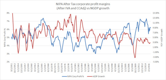
2. If NIPA corporate profit margins did NOT see the same decline in margins that would be support that reported earnings were sandbagged.  The BEA does not rely just on reported earnings but uses tax filings and other data sources, that rely on a different set of accounting standards less subject to manipulation and better represent the actual economic earnings power of corporations.  In addition the NIPA data is much broader encompassing but publicly traded and privately held corporations of all sizes.  This is why I use this data in my investing models.

3. Finally if reported margins in 1Q’19 bounced right back to prior levels it would strongly imply that the 4thq was an anomaly of some sort and this theory could provide a reasonable explanation  

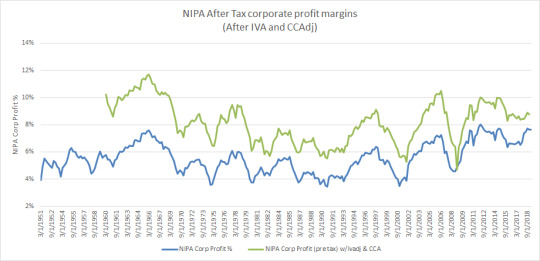
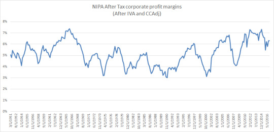
So what do we know?  We know that NIPA margins did NOT show the same decline in corporate profits

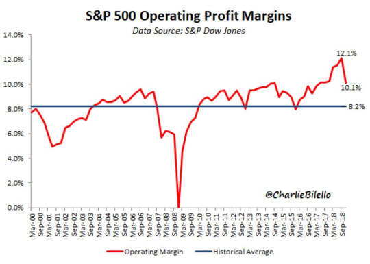
We now also know that reported 1Q earnings have indeed miraculously recovered and that revenue growth has not been robust relative to estimates.  Official S&P data, reflecting a blend of reported and estimated margins, already indicates that operating margins (as depicted above), have rebounded to above 11%.  That figure will settle in higher, possibly approaching levels seen in the 1st 3 quarters of 2018. Here is the link to the current Dow Jones S&P 500 data.  https://us.spindices.com/documents/additional-material/sp-500-eps-est.xlsx

This evidence strongly supports the thesis that the 4thQ’18 was an anomaly, for what ever reason, and I put forth that this theory is a reasonable and plausible explanation.  Unfortunately to many, and I concur, this is a theory that can never really be proven as you would have need to be inside the close processes of all the companies to really know what was happening and how earnings were actually printed.

It is also interesting to note that this process of how earnings get booked is exactly why I don’t use reported earnings in my Longer Term secular trend  model.  Others have noted that reported profit margins LAG NIPA profit margins.  https://seekingalpha.com/article/4249006-eyes-nipa-profit-margins.  The mechanics of that are that when the business cycle turns most companies don’t know it’s a broad turn.  They attempt to continue to report earnings that are at least close to expectations and in the process they empty out latent conservatism in balance sheet estimates.  They can do this for a few quarter and when it becomes plainly obvious that what they are experiencing is a broad end to the business cycle they are forced to report more accurate numbers culminating, usually at the bottom, in a “kitchen sink quarter”  where all bad news is recognized and a much more conservative balance sheet is established and the cycle continues.

Looking forward

The way this game works is that companies never let good news out into their earnings in one big chunk if they can help it.  In all likelihood there will be a steady tail wind to earnings through the year as the conservatism built into balance sheets in 4q’18 gets bled out into the P&L in 2019.  Most notably once we get to 4Q 2019 the Year over year comps are going to benefit substantially from 2018 sandbagging and possibly lead to a smaller repeat where companies that capped out incentive comp plans take a conservative approach to earnings estimates.  Mind you this would be far less companies, in all likelihood far less noticeable.

[pkreilly]

2016 Year in review and 2017 outlook

Please take a look at last January’s year in review and outlook as well as the mid year update and the post describing the model its self for additional context ( https://www.tumblr.com/blog/pkreilly)

2016 Review

In 2016 the S&P 500 broke out of a year and a half period of sideways action punctuated by periods of extreme volatility.  This year end break out was not the outcome expected nor positioned for by the model leading to serious under performance during 2016 (see below).

At the end of 2015 the model was positioned modestly short at (27.5%) based on tepid nGDP growth, Corporate profit margins that peaked at 7.3% in late 2014 and had dropped to as low as 6.6% (all based on revised data).  The fact that SPX was still below Fair Value (FV) of the model meant that despite the modest deterioration of the macro drivers of market behavior that the model was not going to get very aggressive on the short side and that with any declines that the allocations might even flip long.  This is precisely what happened in January-February time period.  As the market retreated the Relative Valuation (RV) dropped low enough to flip allocations to a modest long, as much as 25%, and helped create some gains that cushion the absolute performance during the remainder of the year as the market recovered.

The continuation of the macro conditions of 2015 in 2016 ensured that the model would stay short throughout the remainder of 2016, spending most of the year at 50% short even as SPX became progressively more over FV, only getting more aggressively short into the December time period and ending the year (90%).

So what happened?  In short, and as previously discussed, this environment  is the most susceptible to this type of model under performing.  The 9.5% increase in SPX this year was unexpected and but by no means unprecedented, however it did leave SPX >28% over the model FV. During 2016 what happened is that margins stopped declining and in fact recovered to some degree in the 3Q of 2016 at the same time that nGDP continued to inch up in the 2-3% range through 2016.  This environment of fluctuation in margin performance from quarter to quarter and no strong secular trend is what causes this model the most problem.  I had built in logic to try and minimize model whipsawing but ultimately the burden of proof of what the secular direction for the market is on the bears.  In other words the market is presumed to be in an uptrend unless the macro trends (nGDP and margins) can prove its bearish.  In 2016 they had JUST met those thresholds, established via back testing, keeping the model on bearish footing but it was never the strongest bear case versus other historical precedents.

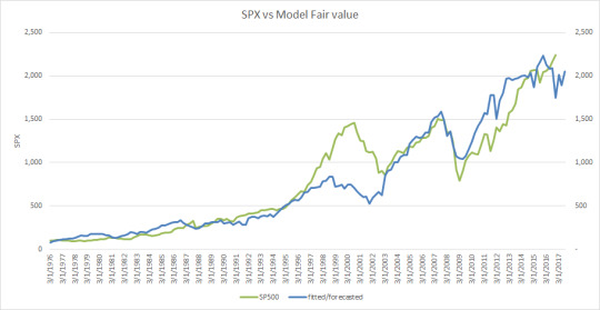
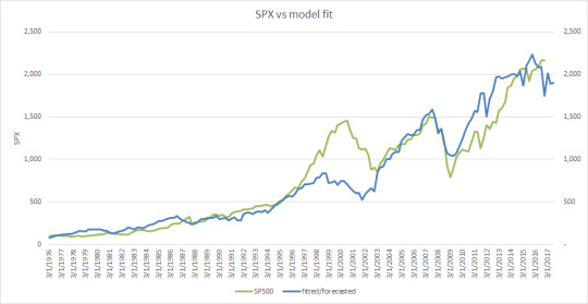
This can be illustrated by reviewing the following chart comparing SPX to the model FV

As should be obvious the last two secular bear markets had much steadier and sustained down turns in the models FV.  This more recent time period beginning in 2013 has been a leveling out of the FV punctuated by margin induced volatility.  In other words nGDP continued to advance enough to provide macro cushion to a modestly deteriorating margin environment.  The following chart shows the corporate profit margin series from the BEA.

2016 Results

2016 was a difficult year for the model logging a loss of (3.3%) and under performing the SPX index by (11.7%).  This represents the first loss back to back loss for the model either in practice or in back testing though the 2 year cumulative loss of (6.5%) is very modest historically in an absolute sense AND in the context of the gains generated during the aggressively long positioning during the 2011-mid 2015 time period.  The nature of this model is to identify the secular trend in place, and the one that will likely continue to be in place, and ride that trend in a levered fashion.  The impulse less environment we have experienced since 2015 is relatively unique and provided no secular trend that was clear.  This is precisely the type of environment where my model should under perform.

These results are tracked via my, mostly, daily end of day model positioning tweets.  The public history is documented in this way and summarized here:

https://1drv.ms/x/s!AnPYhvrUKocWdXIyYVOcC9w_-8s

these performance figures require caveats, including:

1.  SPX dividends are not included

2. Any yield from cash held by the model are not included

3.  transaction costs are not included but are fairly de minimus given the secular positions taken

4.  gains from frictional changes to target leverage due to changes in the delta of the options used in establishing the target portfolio are not included

5.  The calculation presumes that the position is established at market close through the next day.  there are in fact gains generated from managing the portfolio’s options to the target delta.

2017 Outlook

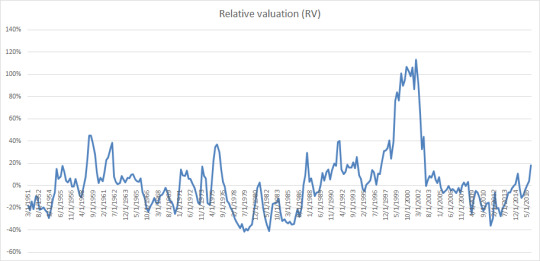
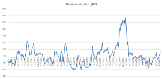
At the end of 2016 the bears no longer have the burden of proof on their side, margins have stopped declining, modest past nGDP growth continue to provide some valuation support. this means the model will flip to a more aggressive allocation scheme in 2017.  However things are no all peaches and cream.  The late 2016 advance has left the SPX at relatively high valuations for the macro underpinnings.  This once again leaves the model exposed to more whipsaw action.  The macro pulse is still weak and the up turn in margins is nascent and could still be subject to volatility.  For example a mere 50BP drop sequentially in 4Q16 NIPA corporate profit margins would flip the allocation rules back to a more cautious and even bearish stance.  More over with the 1H’17 model FV  in the 1900 to 2050 range SPX is over valued but not wildly from a historic perspective.  This chart of historical RV’s (extended to 6/30/17 at year end SPX prices) illustrates that.

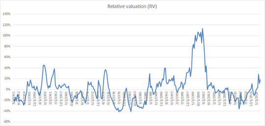
So where does that leave the model?  The model will be transitioning over a 10 day trading period to the more aggressive allocation scheme per model rules.  At these prices and RV that would leave the model 65% long in 2 weeks.  At these prices  at quarter end and the recovery in the FV of the model the allocations will be transitioning to a more levered position (>100% long).

The risks in all of this is that we have the following conditions:

1. Still no solid secular trend, merely a default to a more bullish stance as the bears lost their proof

2. market is over FV but not wildly so in 1H 2017

3. the potential for more whipsawing in the assessed secular trend direction

All of this leads me once again to be very concerned about model under performance.  However, not that worried, as this is an unusual time period.  The Macro drivers WILL become clearer over time and that is where the model shines and produces out performance.  Until that time patience is warranted.  What happens though if we are in a new normal of much lower nGDP growth and stable or even continued declines to margins over a multiple year time period? In short this model will under perform the market as will the vast majority of trend following models, whether fundamental ones like this, or technical analysis based ones.

For the record the current year model FV is 2,060 and I will adapt that as the provisional 2017 YE target subject to updating as more data about 2016 emerges and the potential, as always, that annual revisions to the NIPA series in mid year change the model FV.  I know this sounds illogical given the bullish posture the model is about to adopt but past history indicates you need to be long in the absence of definitive bearish secular support.

2018

Given the dominant role of changes in corporate profit margins and the lag time in which the market reacts to them very little can be said of 2018 prospects.  However the lead time of turns in nGDP to turns in SPX does say that the ongoing modest growth in nGDP does provide some valuation support for growth.  If margins stay stable a model FV of 2100 to 2200 in CY 2018 would emerge allowing the potential for staying long but also the potential for extreme over valuation conditions to emerge is SPX continues to advance over this time horizon.

Best wishes in the new year!

Peter

[pkreilly]

VXST ST model

A few months back Dana Lyons from JLyons Fund Management publish a blog post noting that big drops in the CBOEs Short term option volatility measure, VXST, appeared to provide reliable buy/sell signals.  This blog post will discuss what the VXST is, examine further why it might provide signals in the way that were discussed by Dana, discuss some tweaking I have done and discuss why I withdrew the sell signal from my daily tweets, for now.

VXST what is it?

VXST is the CBOEs short term version of VIX, the volatility index.  From CBOEs website it succinctly describes the VXST

“ The CBOE Short-Term Volatility Index (VXST) and the CBOE Volatility Index® (VIX®) both reflect investors' consensus view of expected stock market volatility. While the VIX measures expectations of 30-day future volatility, the VXST provides a market-based gauge of expectations of 9-day volatility, making it particularly responsive to changes in the S&P 500® Index. The VXST Index provides a market estimate of short-term expected (implied) volatility that is calculated by using real-time S&P 500® Index option bid/ask quotes. VXST uses nearby and second nearby options with at least 1 day left to expiration and then weights them to yield a constant, nine-day measure of the expected volatility of the S&P 500 Index. “

The very nature of volatility indices is that they are TWO WAY composite indices of the price of options, at various times to expiration.  The VXST is a 9 day composite pricing of Calls and puts.  Many people mistakenly view these indices as one sided, reflecting only the risk of the market dropping.  Option premiums and therefore volatility indices can be bid up in bullish situations as demand for calls accelerates, as we have seen recently.  This can be ferreted out by various skew and option P/C ratios.  These circumstances can be reflecting acceleration of sentiment, sometimes in a lopsided way.

Other times volatility indices can drop rapidly as the fear evaporates after a healthy pullback in the market.  If the VIX drops rapidly close to the highs of the market it can reflect the exhaustion of call buyers, signalling the potential for a pull back.

The model

The basic logic of the model that Dana published is that big drops in the VXST when you are far away from 52 week highs are bullish and big drops when close to or at 52 week highs are a least neutral or possibly bearish.  I view the differentiation of being close to 52 week highs or not as proxy for distinguishing whether or not run ups then drops in VIX are due to call buyer exhaustion or put buyer exhaustion.  It’s quite possible there are more direct measurements or indicators that when substituted would produce more accurate, granular signals. The specific parameters of what it means to be far away from 52 week highs and what are “large” drops were discuss in Dana’s original blog post found here:

http://jlfmi.tumblr.com/post/150770836985/traders-quickly-get-comfortable-with-stocks-again

Needless to say I tweaked the parameters a little explored what the optimal back tested logic was, extended the history of VXST back to its origins.  I wouldn’t say my parameters are profoundly different from Dana’s but there are different.  I also explored whether changes to VXST to the upside provided any potential signal and could not find that relationship.  Here is a graph of all the bullish and bearish (Neutral?) signals.

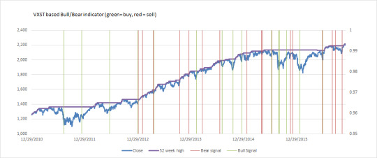
The models signals are based on closing prices of the market and VXST and strategies are implemented at the close for back testing purposes.

Results and strategies

So what should be obvious is that since the inception of VXST that large drops away from 52 week highs are flat out money calls.  Large drops close to 52 week highs are more mixed.  In back testing adopting it as a bearish signal does add to the model performance relative to SPX but not nearly as much as the buy signals.  In fact most of that comes from only a small handful of bearish signals. the market has been on a bear signal since 9/9/16 yet we are at ATH’s, though nominally so relative to when the first bearish signal was triggered On the bull side it appears that it is a buy at will signal and the use of leverage seems warranted and limited only for your tolerance for draw downs.

In back testing if you adopted the strategy of going long when model is in bull and 100% cash when in bear you would have outperformed the SPX by 2.4%/year compounded a not insignificant feat.  If you went 100% long on a bull signal and 100% short on a bear signal you would have out performed by 4.8%.  If you used 2 times leverage during a bear bull phase you would have outperformed the market by 15.4% compounded. If you added 2 times leverage on bear signals you out performed by 21%.  Note that the adding of leverage on the bullish side amps returns far more than adding on the bearish side reinforcing the point about the relative strengths of the signals.

I will note that I have also back tested this model in conjunction with my Long Term secular trend model and the two work together well, adding to out performance in back testing.  If either model were noisy or aberrations one would expect the potential that the market positioning might interfere with each other and reduce or eliminate out performance.  That is not what I found.

Conclusions

Its because of the uncertainty around the bearish signal that I withdrew this model from the public, for now.  The VXST still has limited history and the potential that this “signal” is the result of statistical noise and found through brute data mining is real, despite the rational for the triggers to exists.

My intent is to not include this model with my LT model tweets just yet but I will note when significant signals emerge.  My intent in my personal portfolio is to take action on the bullish signals and to watch the bearish signals for now.

Peter

[pkreilly]

Latest Model Update (11/29/16)

Today the government released updates to 3Q’16 GDP estimates which modestly revised upwards the growth rate of nominal GDP (nGDP).  More importantly to the model the first look at economy wide corporate profit margins for 3Q’16 were released and these indicated that the declines in profit margins have abated and this will result in the model flipping back to a long position 1/1/2017.  Please take a look at the previous blog I wrote on the Long Term Secular trend model and it’s workings for more detail.  The model is not  a trading one but one that takes long term (multi-quarter and multi-year) secular positions and often will use leverage if the circumstances are right to try and generate excess absolute returns.

Here is a chart of the profit margins that are part of the underlying FV model:

Note the peaking and then stabilization.  The lack of follow through to the downside is why this is not yet the secular bear market that many seem to having been expecting/hoping for.  That doesn’t mean it cant develop but the history proves that the burden of proof is on the shoulders of the bears and if they cant prove it then the tendency is you have to be long.

It is worth noting the the LT model has been short (50%) since the 4th quarter of 2015 when SPX was trading around 2030.  With SPX up almost 10%, and the painful under performance over that period, and SPX more overvalued you might ask (and others have) why the long signal?  Well in short the model uses logic that if the predicted future Fair Value of the SPX isn’t declining and its not TOO far above that FV then you should position long.  Not nearly so much long as if FV was rising AND SPX is <FV.  This time period, the past 2 years, period has been a tough one precisely because there has been little secular trend and what one there has been for the model FV has been flat down.  It’s pretty much the worst case scenario (except 1999-2000 where the model was short too early) S&P 500 spent much of the past 2 years chopping within a relatively narrow trading range while the 4th Q of 2016 is turning out to be the NADIR for the model fair value.  Only now is the market breaking to new all time highs.

This chart illustrates the SPX vs the model FV:

The take away’s from the chart are:

1)  Model FV peaked 4Q’15 (after revisions to nGDP changed the timing a bit which is why the model in practice started getting short in 4Q’15).  As the model FV began to flatten and SPX became more fairly valued the market went into a period of sideways consolidation marked by some violent pullbacks.

2)  Model FV dropped substantially creating the situation where the model logic for determining whether it was dropping triggered, yet it has subsequently stabilized and has recently been showing a nascent upward trend.  Don’t forget that the heart of this is a PREDICTIVE model for SPX FV.

3)  Market is overvalued relative to the FV but not unusually so from a historical perspective (see the chart below)

4)  The market CAN continue to get more over valued and based on the history of the model this is what allows the model to be long, but not terribly so and in diminishing amounts of  SPX continues to rise.

5)  There is ongoing risk that the whipsaw logic of the model will continue to be tested.  The upward trend of the model FV is not strong and it is not well established AND the market is over valued.  It would only take a 30BP decline in NIPA margins sequentially to throw the model back into bearish model later in 2017.  In other words this is still not an optimal environment for excess returns for the models approach.

6)  If SPX does correct on the macro fundamentals remain supportive (ie growing nGDP and corporate margins that are a least stable then the long case is strengthened. If SPX continues to power higher but margins turn down from here it might actually set up a more aggressive short opportunity in the 2H.  But these are just what ifs for now.

Good luck and as always use this work at your own discretion.

Best wishes Peter

[pkreilly]

Portfolio management using options

In my previous blog I referenced my portfolio management strategy as using options to target desired leverage using a bar bell strategy.  Someone suggested this might be a good topic for a blog post so here goes.

If you have a process that sometimes calls for leverage to be used, one alternative, among many, is to use options.  I use options on SPY ETF as the underlying is highly liquid as well as the options markets.  Options allow you to generate leverage, incurring the cost of option premium decay but allowing you to confidently own the position without margin calls (there may well be funding needs however to maintain your desired market exposure as the underlying moves, this will be elaborated on below).  The use of options allows you to keep large amounts in cash while obtaining your desired leverage or positioning. It does require you to make adjustments to the portfolio regularly to maintain desire exposure to the underlying as the price of the underlying changes.  It also subjects you to decay of the option premium but this can be mitigated as part of the process using carefully chosen expirations and through the trading required to maintain a target market exposure (delta in other words).

Some option Basics and terms

I don’t propose to write a primer on options and I presume you have some familiarity with the concept but its worth going over some key concepts.  First is that of premium, the price you pay for the right to buy or sell the underlying at an agreed upon price (the strike price) within an agreed up time (expiration).  That premium is a function of how far away that agreed up price is from the actual price of the underlying, the amount of time left on the contract and the expect volatility of the underlying over that time period.

The next key concept is delta, the amount the option will move at the current conditions (they constantly change with price and time) with a move in the underlying price.  for example if the delta is .5 then the next % price movement of the underlying should produce a .5% move in the option.  As the underlying moves towards and then beyond the strike the delta increases assymptotically to 1.0 in a non linear way.  As time passes and the option premium decays delta will increase if the underlying price is beyond the strike price and decrease if it is not.  Finally if the volatility of the option is repriced to new levels the delta will also change.  

The key take away for delta is it is what gets you exposure to the underlying asset price move and that is changes often driving the need to adjust the portfolio to maintain your target market exposure.  As the price of the underlying moves in the direction your positioning expects then you will GAIN delta typically requiring you to sell instruments to maintain the target (presuming the target exposure of your process doesn’t change).  The opposite is also true that if the underlying moves away from the direction expected you will typically need to buy more delta to maintain target exposure.  This process driven by movements and often price gapping of the underlying produces trading gains that can help offset the decay of the option premium over time.

Leverage & Options

I want to lay out what I mean by leverage and describe how to think about the leverage that options produce.  Leverage is the control of more assets than your money would control on a $ for $ basis.  Leverage is sometimes achieved through margin borrowing, sometimes through futures and contracts, but options also act similarly.  If you buy 1 option that gives you the right to buy 100 shares the S&P 500 ETF SPY for $5/option or $500, SPY trades @ $215 and the option has a delta of .5 then you effectively control $215*100*.5 or $10,075 of SPY.  This option produces leverage of 21.5 to 1.

Bar Bell Portfolios

A bar bell strategy is one where you aim to gain desired leverage while maintaining high levels of cash that may be invested conservatively to generate some yield that you would have generated by holding the underlying but have foregone through the use of options.  It also can be though of as generating some yield to offset the options decay.  The exact mix of options, their strike and expiration vs the amount of cash held depends on the underlying strategy you are pursuing.  This approach to portfolio management is well suited to mean reverting strategies where you want to gain exposure the further the underlying moves against your expectations.

The exact leverage you hold is the weighted average in $ terms of the cash held (which has no leverage to the underlying or 0) and the value of the portfolio of options.

The following table illustrates this concept:

This is a $1M portfolio which is 80% in cash and @ (146%) levered short (or 1.462 times short).  What should be clear is that the delta of the options are a key component of how much leverage they have.  This is why as the delta moves (due to price movement, time or volatility changes) portfolio adjustments or trading is required to maintain a target levered exposure.

Conclusion

I hope this was helpful and illustrative.  It is not a recommendation for anyone to use these concepts as it may not be suitable for your strategy.  For example any strategy that changes positioning in the opposite direction due to changes in the price of the underlying (ie you flip from long to short as price deteriorates) as would often be the case in many trading methodologies.

However in mean reverting strategies where you don’t want to be forced out of a margin or futures generated levered position when the underlying goes against you it may be appropriate.  It is also worth noting that while apply these to SPY the concepts are directly applicable to any underlying instrument.

Peter

[pkreilly]

Secular SPX Trend Model

So enough people see my posts on twitter about my model that I felt it was important to post an over view of the Long Term Secular model.  The model has two components, one a statistical model that uses nominal GDP and corporate profit margins from the National Income and Products accounts data set (NIPA) to estimate the Fair Value (FV) of the S&P 500.  The second piece is the logic for determining whether that FV is in an up or down trend and how to position an aggressive portfolio based on the model.  

The Model

The model is relatively straightforward but with one key twist.  My work has found that there is a leading indicator relation of turns in the economy and economy wide corporate profit margins on the stock market.  In other words there is a predictive period in which the market follows turns in the economy, creating exploitable value.  The model itself uses only those two variables.  Its key to note that know the FV does not get you much as SPX can deviate wildly from that FV, becoming over and under valued for long periods of time.  This is where the maxim “the market can stay irrational longer than you can stay solvent” comes from.  Many people have gone bankrupt shorting over valued markets.

However when you add in the ability to predict the FV, or center of gravity as I sometimes call it, it adds a second key dimension.  What I have found is that its not just the relative valuation (RV) of the market that matters but the DIRECTION that FV is trending in and will continue to trend in.  

The Model Rules

In order to take advantage of the inherent predictive value in the core model I recognized that you needed two things:  Logic to determine if the FV was really in a downtrend vs an uptrend.  You can consider this whipsaw rules and in general the weight of the evidence has to be on proving that the a secular down trend is real.  Once you determine whether the market  FV is in a secular down trend or uptrend I then determined optimal portfolio positioning along two dimensions: one the relative RV of the SPX and whether FV is trending down or up.  In general the lower the RV the more aggressively long and vice versa.  Also when FV is in an uptrend the model is longer at higher RVs and vice versa.  It is possible to be long despite high RV as long as the FV is trending up.  It’s also possible to be short if RV gets high enough, despite a rising FV.  Conversely with a declining FV its possible to long if RV gets low enough.

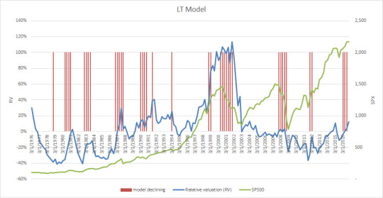
The following chart illustrates the SPX over-layed with RV and periods of declining FV.

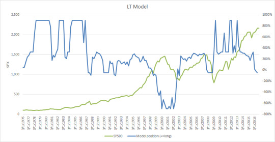
The next chart illustrates the historical model positioning vs the the SPX

History and application

I began developing this model in 2010 and have been refining it consistently.  For example initially the second dimension of of the model didn’t exist and I was investing solely based on the RV.  In addition I developed and refined the logic around what FV was doing. 

The model in back testing compounds out at >70% from the 1976-2016 time period but these aggressive rules are subject to significant portfolio volatility and sometimes material draw downs. This is using purely mechanical rules with no judgment affecting positioning (only the precise mix of instruments to achieve market exposure) It is possible to apply less aggressive versions of the portfolio positioning.  I have been using the model since early 2011 with good results, though the past two years the market has been relatively trend less which is the worse scenario for the returns. (see my other posts on the market outlook informed by the model)

Portfolio Management

Given the aggressive nature of the rules I apply portfolio management is critical as the possibility of “ruin”, where severe draw downs impede performance.  In particular the source and generation of leverage is crucial.  In general I use a bar bell portfolio strategy where I hold lots of cash and use option portfolios to generate target market exposure.  This means that the portfolio is managed to a target delta to maintain model exposure to the market.

 I use the model currently to manage my own money and may one day apply it professionally under the right circumstances.  My background is in Math, Statistics, Economics and Actuarial Science.

[pkreilly]

Updated 2016 Outlook

Fridays release of final 4Q’15 GDP along with the first view of corporate profits across the economy marked a major shift for my model.  The model uses nominal GDP and corporate profit margins, with independent lags, to PREDICT the fair value of SPX for some period in future.  With a significant drop in corporate profit margins I am establishing my Year end price target (FV) of 1756 and the model will remain in the more conservative portfolio rules until at least year end.

To recap the past few years corporate profit margins (after after tax with inventory valuation and capital consumption adjustments) peaked in late 2011.  However they did not experience a significant decline immediately, allowing for market support from ongoing, but modest, rises in nGDP. That began changing notably in 1Q’15 with more pronounced declines in margins.  This put the model in a defensive posture and the ongoing declines in margins is leading to declining support for current valuations.  The period after the peaking of margins has been characterized by sideways (and up and down) market action with flipping of the model between conservative and aggressive model rules.  In others words pretty much the worst environment for the model to out perform.  Notably in 2015 the model had it’s first loss (in backtesting or live use) since 1999.

It’s important to note that markets do not have to reach significantly over valued levels to decline.  The issue is if either nGDP or margins turn (or both) this LEADS to declines in SPX and markets can fall from currently reasonable valuations.  This is the situation we are likely to find ourselves in in 2016.  That does NOT mean that markets will decline immediately but positioning now in the model is short 50% for an anticipated decline later in the year.  At a minimum the enironment does not support markets advancing materially and if they did it would lead to the potential for a more meaningful (ie >50% short) opportunity under the model rules.

Its also important to note that even if the model FV bottoms at that level markets can and often due over shoot to the downside when FV is declining, creating a meaningful long opportunity when FV bottoms and turns.  This is the environment where my model produces the vast majority of absolute returns, though it does produce generous RELATIVE returns during bearish timeframes.  Whether or not this is the bottom for FV is yet to be determined but what is clear is this is the most bearish development in the model since it went bearish in the 4th quarter of 2007.

Buckle up and best wishes.  Peter

[pkreilly]

2015 Year in review and 2016 outlook

2015 Review

After a good 2014 where the markets ended within 1.0% of my revised target for SPX of 2050, and the model returned over a 30% gain, I published my initial SPX target for YE 2015 at 2001 in early January.  The basis for this, driven by my proprietary model, was the lack of strong growth in nominal GDP and a peaking of corporate profit margins, broadly measured in the NIPA data.  This represented an expected decline in the S&P500 index of about (3.0%).  This view was complely out of step with the general consensus that a high single or low double digit gain was in store for the markets, in other words more of the same. In the middle of the year, in reaction to data revisions released in late August my YE target was revised to 2087.  The SPX ended the year at 2043, below this revised target but smack in the middle of the initial estimate and the final estimate.  Being within 2% of the final index level, while not quite as good as previous years is still quite good performance.  In either case the investment conclusions published last January that this year would be a year of consolidation and directionless market activity, punctuated by volatility was spot on (please refer back to my 2014 year and review and 2015 out look https://www.tumblr.com/blog/pkreilly )

Entering 2015, based on the projected change in market FV over the next year, which was down, the model portfolio allocation was short (27.5%). However in my 2015 outlook I made it clear this would not hold as a move to a long position as of 4/1 was ordained by stabilization of margins in 2014. As the year evolved a few significant developments occurred that had meaningful effects on the models expectations for SPX at YE 2015 and moving into 2016.  The first event was the release of 1Q'15 corporate profits in May.  This release saw a significant drop in profit margins in the National Income and Product Accounts (NIPA) Corporate Profits after tax and inventory valuation and capital consumption adjustments.  This is the series I use in my model as it best represents the economics of corporate america. The drop was primarily due to the lapsing of certain tax credits, however even without that margins have clearly stopped expanding in the NIPA data.  The implications for the future of the stock prices if the lower margins persist would be negative, lowering the fair value of the market, and the current short position of the model is due to this meaningful drop.  In fact the lower corporate profit margins did persist in 2015, but crucially they have appeared to have stopped going down after 1Q, at least through the 3rd quarter.  This pattern of fluctuation without a persistent quarter to quarter change in direction, against the backdrop of persistent, if modest, growth in nominal GDP, is what is creating the uncertainty as to the actual secular direction of the market.

The next significant event came in late July with the 2Q GDP which included the 2Q corporate profit margin series and importantly the annual revisions.  these revisions upwardly revised coporate profit margins over the past few years and lead to an increase of the model fair value at year end to 2087.

2015 Results

2015 was adifficult year for the model logging a loss of (3.2%) and underperforming the SPX index by (2.5%).  This represents the first loss for the model since 1999.  However this result was not wholely unexpected given the lack of strong impulse in either direction and the whipsawing of the model between long short positions intra year.  I did create and back test adjusted rules to minimize the chance of whipsawing and it did increase back tested returns.  However even that was not enough to forestall underperformance in this unusual environment.  The nature of this model is to identify the secular trend in place, and the one that will likely continue to be in place, and ride that trend in a levered fashion.  The impulseless environment we experienced in 2015 is relatively unique and provided no secular trend that was clear.  This is precisely the type of environment where my model should underperform.

2016 Outlook

2016 appears to more of the same, low nGDP growth historically high, but stable margins leaves the market impulseless.  2016 is by no means written yet but there is no indication of a secular turn coming, yet no room for growth in the averages except from multiple expansions.  This is setting up another volatile trading oriented market with opportunities to sell option premium (puts and calls) around a broad range of the S&P 500 (1850 to 2150).  If the market drops to the low end of this range getting long may make sense and at the upper end of the range greater caution.

The enviornment not supporting signficant growth in the SPX doesn’t mean it can’t happen, it’s just less likely based on my work.  A significant rise in the SPX would lead to increasingly over valued conditions, yet it takes markets to be >20% above fair value for my model to get shorter than 50%, so it would take a pretty stellar rise to create a “big short” like situation, and even great increases to get short while FV is trending up (not very likely to happen in 2016).

What about significant declines?  Again not terribly likely unless economy wide margins continue what was started in late 2013 and resume their declines from the lower but stable levels as of 3Q’15.  Again that doesnt mean SPX couldnt revisit the 1800′s during the year but at this point that should be viewed as a buying opportunity, as my model rules would view it.

3Q'16 model FV is approximately 1986 or about 2.8% lower than YE 2015 and I am establishing this is as my YE 2016 price target, on a preliminary basis.  the final YE target will be set in April and revised in July (with the annual NIPA revisions).

At this stage the model is implying a period of weakness in the 1Q time frame and model rules are positioned with a short exposure heading into 2016.  However given the stabilization of margins and continued growth in nGDP in 2015 this will not persist and the model will flip to a long position again in 2Q'16.  The potential that this is just more flip flopping is quite real and the environment once again in 2016 is not one conducive to out performance.

The risks to this 2016 outlook are that the market could resume going up solely because that is the markets tendency with out a distinct secular downturn in margins or nGDP (or both).  This would lead to the market becoming overvalued but not meaningfully change the models positioning as it will go long 4/1, its just a matter of how much (based on the position of SPX vs model FV).

2017

Given the dominant role of changes in corporate profit margins and the lag time in which the market reacts to them very little can be said of 2017 prospects.  My model indicates that on average the market reacts much more slowly to turns in nominal GDP, possibly due to the lag time of revisions.  The ongoing growth in nGDP does provide valuation support into 2017 but the year will be driven by action in corporate profit margins.  The implication though is that a true secular downturn in the market is still less likely due to the valuation support provided by past nGDP growth.

Review of the Model

The valuation model relates the SPX index to the size of the economy (nGDP) and the profits that corporations (of all sizes) extract from the economy (corporate profits, after tax and with capital consumption adjustments and inventory valuation adjustments).  The model reflects that nGDP and corporate margins LEAD the SPX and there produces some predictive power for the future path of the long term fair value (FV).  Investments rules were constructed based on the position of SPX vs the FV AND the predicted direction of the FV.  In back testing these rules produce superior returns to by and hold unlevered.  In their most aggressive form, which I apply to my personal investment account, they produce compounded annual returns of 72.6% (back tested) to 1976.  

In 39 years of back testing, up to and including 2015, the model has produce negative returns in 5 years, 1977, 1978, 1981, 1998 (slightly negative) and 1999 and now 2015.

Some of those draw downs were quite large but the 1998 & 1999 negative returns came after riding the bull market in a highly levered way and the draw downs are only large in absolute but quite small in relationship to the gains that preceded it.

Best wishes in the new year!

Peter

[pkreilly]

2014 Year in review and 2015 outlook

2014 Review

After a spectacular 2013 where the markets ended within 1.0% of my target for SPX of 1865, with over a 30% gain, I published my initial SPX target for YE 2014 at 2150.  The basis for this, driven by my proprietary model, was the ongoing growth in nominal GDP combined with the margin expansion in the economy that had occurred in 2013.  This represented an expected growth in the index of about 16.0% and was above all targets coming out of the major market analysts.  There was wide discussion at the time that when you have a 30% type gain, as in 2013, the next year is typically a pretty good one with returns in the mid teens.  My target was not driven by this fact but was consistent with that and 2014 has come very much in line with those returns ending the year at 11.4%.  The SPX ended the year close to my revised target, ending up at 2058.9, very close to my revised YE target of 2050, published in August.

As I published my target for SPX I described a year that was likely to have much more trading opportunity from both the long and short side as almost every normal year in the market has at least a few significant draw downs of >5% and 2014 saw meaningful drops in February, August and October. In order to get an annual return of 16% along with three draw downs like that you mathematically need more variability and once again 2014 cooperated quite nicely with this view.

Entering 2014, based on the projected change in market FV over the next year the model portfolio allocation was 321.8% long.  This was down from over 400% long at the beginning of 2013 as the market become far less undervalued.

As the year evolved a few significant developments occurred that had meaningful effects on the models expectations for SPX at YE 2014 AND moving into 2015.  The first event was the release of 1Q'14 corporate profits in May.  This release saw a significant drop in profit margins in the National Income and Product Accounts (NIPA) Corporate Profits after tax and inventory valuation and capital consumption adjustments.  This is the series I use in my model as it best represents the economics of corporate america. The drop was primarily due to the lapsing of certain tax credits, however even without that margins have clearly stopped expanding in the NIPA data.  The implications for the future of the stock prices if the lower margins persist would be negative, lowering the fair value of the market.  However for this to be true the new lower margins would need to stabilize at the new levels. Further drops would imply much more risk to the downside and a subsequent rebound would blunt the negative implications.  The model meanwhile maintained a recommended exposure of approximately 320% and the market had made very little progress YTD. Bearish commentators were widely touting the lack of return on the SPX at this juncture.

The next significant event was the 2Q'14 GDP release in late July and was accompanied by the annual revision of GDP and corporate profits.  This was a very significant event in the profit margins, economy wide, were revised downward back into the 2nd half of 2013, indicating that the turn in profit margins had started earlier.  This development heightened the future risk and accelerated timing of the potential impact.  YE 2014 SPX target was lowered to 2050 at this time based on the model and my judgement that the market getting all the way back to FV was not likely. The model FV moved to 2102 with the new data. At this stage I began discussing the potential for a meaningful turn in the market near year end and into 1H 2015.  Though the model rules based on the available information and the timing of the risk were still long, well over 300% and got longer into the August declines.

The next significant event came in late August with the second revision to 2Q GDP which included the 2Q corporate profit margin series.  This indicated that profit margins rebounded only modestly in 2Q and that the reduction in model fair value was more likely to be persistent despite the continued growth in nominal GDP.  At this juncture, due to the projected decline in the model FV for the next 2 quarters, the model rules flip to a much less aggressive stance.  I also did some additional back testing of the model rules which let to some restructuring of the rules for better back tested performance.

As of late September market exposure had been greatly reduced.  However the significant sell off in October led to the model flipping back to a levered long position despite the projected turn.  The market had just fallen far enough to skew the risks to the long side.  From there on market exposure has been steadily reduced and the model flipped to its first short exposure since I built the process and short exposure has ramped up to 27.5% as of year end.

The final significant event for the model was the release of 3Q'15 corporate profits which once again showed some improvement off the 1H'14 levels.  The implication of this is that the turn in model fair value is going to be short lived and the implied risk in 1H'15 should be relatively modest in depth and transitory in nature.  In fact, no matter what the SPX does in 2Q'15 the model will shift back to a long position

2014 Results

2014 was another great year for the model. Given the 11.4% annual change in the index and the very long exposure through much of the year the model portfolio once again outperformed the S&P 500 returning 31.2% or 17.75% in excess of the SPX.  The model portfolio actually continued to produce positive returns despite the more cautious stance as the October dip was bought producing some trading gains.  However some relative performance vs the SPX was lost in the final few months as the SPX continued to climb and finished the year in excess of my revised YE target but below the initial target set in early January.

2015 Outlook

2015 will quite likely be a more difficult year for the market.  The turn in economy wide corporate margins are setting the stage for at least a consolidation year and the possibility of outright year over year declines.  

There of course will be long and short opportunities within the year and volatility will likely be much higher within the year and while I hold no official position on the VIX, the implications are that volatility should be owned.  

3Q'15 model FV is approximately 2001 or about 3.0% lower than YE 2014 and I am establishing this is my YE 2015 price target, on a preliminary basis.  How the SPX gets there could be quite interesting and frankly there is some chance that the market doesn't decline and merely consolidates.  In either case the investment conclusions are very similar.  Given the model implies more weakness in the 1st half its also possible we get a meaningful correction, say under 1900 and then the rest of the year is spent stabilizing and recovering. 

At this stage the model is implying a period of weakness in the 1Q-2Q time frame and model rules are positioned with a short exposure.  However given the stabilization of margins and continued growth in nGDP in 2014 this will not persist and the model will flip to a long position in 2Q'15.

The risks to this 2015 outlook are that the book on 2014 margins are not completely written and it is not at all inconceivable that the market could ignore the possibility for transitory weakness and plow right through the period.  This result, some what confusingly, is that the models rules dictate flipping to long exposure in the 2nd quarter no matter what actually happens in the 1st.  This is due to the stabilization on recovery in the NIPA margins and the continued growth in nominal GDP.  This scenario would lead to SPX becoming overvalued to a meaningful degree as we moved through the year. However as long as the model FV was rising some long exposure would be maintained unless a 1999 like scenario developed.

2016

Given the dominant role of changes in corporate profit margins and the lag time in which the market reacts to them very little can be said of 2016 prospects.  My model indicates that on average the market reacts much more slowly to turns in nominal GDP, possibly due to the lag time of revisions.  However given that slowness the more rapid growth in nGDP now will provide valuation support into 2016.  This makes a true secular turn in the market far less likely unless margins truely begin to contract in a more notable way.

Review of the Model

The valuation model relates the SPX index to the size of the economy (nGDP) and the profits that corporations (of all sizes) extract from the economy (corporate profits, after tax and with capital consumption adjustments and inventory valuation adjustments).  The model reflects that nGDP and corporate margins LEAD the SPX and there produces some predictive power for the future path of the long term fair value (FV).  Investments rules were constructed based on the position of SPX vs the FV AND the predicted direction of the FV.  In back testing these rules produce superior returns to by and hold unlevered.  In their most aggressive form, which I apply to my personal investment account, they produce compounded annual returns of nearly 53% (back tested) to 1976.  The rules have a Sortino ratio (annual calculation) of 520%.

In 38 years of back testing, up to and including 2014, the model has produce negative returns in 5 years, 1977, 1978, 1981, 1998 (slightly negative) and 1999.

Some of those draw downs were quite large but the 1998 & 1999 negative returns came after riding the bull market in a highly levered way the the draw downs are only large in absolute but quite small in relationship to the gains that preceded it.

Best wishes in the new year!

Peter

[pkreilly]

On the nature of risk

As part of my economic and actuarial studies I learned about the Capital Allocation Pricing Model and it’s definition of risk as volatility.  This definition never sat well with me as I could not come to grips with why price fluctuations would be equivalent to the economic risk inherent in the asset. In this blog I explore the nature of risk and layout the conclusions from an investment perspective that I take away.

Risk as Volatility

Prices of assets fluctuate every day.  The casual observer thinks “This is crazy how can the price of a company move second to second with each trade?  How can the stock market go up and down dramatically, surely the underlying economic value of those assets can not alter that much in so short a time?”  The casual observer is dead on as the true economic value is not the primary driver of the “volatility” in prices that are observed every day. 

In order to understand the difference between risk and volatility it is worth stepping back and examining what is going on in markets to drive the movements of prices.  When one examines the process the concept of volatility being risk becomes absurd.

One of the methods I use when explaining or illustrating concepts is to reduce the concept to an extreme or absurd, easy to understand example where the conclusions become obvious and you can then apply to more complicated or subtle situations where the conclusion would not have been so obvious.

If you buy an asset at 90 while your valuation says it’s worth 100 and the price varies between 50 and 99 for 3 years but on the first day of the 4th year it trades at 100 (fair value) and you sell, was the risk really the price fluctuation?  Only if you sold at a mis-priced transaction. So the real risk was not knowing what the proper economic value was.

Valuing Assets

Take it as a given the a particular economic asset has a value of 100 based on the most likely present value of future cash flows.  However participants in a market don’t know that.  They each have a model, or a set of guidelines, or even rules of thumb to estimate the value of the asset.  When a transaction occurs in the market it is because the buyer thinks the asset is undervalued and the seller thinks it’s over valued.  The latest price is a simple result of this matching.  In liquid markets many of these transactions occur each day at varying prices creating the illusion of volatility and risk as clearing prices fluctuate.  What is really at work is the expression of alternative valuations of the assets.  So the asset might be worth 100 but you can get fluctuations in the price from the current state of the market just because of the lack of full information.

The CAPM presumes every agent in a market can value an asset equally well and assimilates information uniformly and instantaneously.  If this were true then the observed market place fluctuations in price would truely be risk.  However the concept that all market participants value assets perfectly and instantaneously is absurd.

Price fluctuations

The observed fluctuation in prices can be thought of having two components.  The first and most important but in most cases not dominant is the actual fluctuation in economic value.  For example a businesses most likely net present value of future cash flows will vary with economic conditions, the particulars of the industry they operate in, the required return of investors to compensate them for the economic risk they are assuming (discount rate), etc.  In other words the inherent economic value of the asset will vary and change over time.  The second source of variability, and I will make the argument that it is the dominant one, is the fluctuations in price due to the inability to accurately value the economic risk of the asset.

So in a market where participants may have wildly differing valuation of the economic value of an assets prices fluctuations make perfect sense.  CAPM envisions a world where information flows equally and instantaneously and where economic value is uniformly estimated.  In this world it makes perfect sense that the observed price fluctuations can only be from fundamental changes in economic value.  However in the real world the valuation of economic value can vary dramatically.  As an example just read the financial press on any given day and there will be expert telling you that the S&P 500 index should be at 1900 and another will tell you it should be at 900.  If the overall market can be viewed so differently imagine how different the valuation of a single security can be viewed.

So price fluctuations also arise from the simple fact that people value the assets differently.  The price of the asset recorded as a transaction is merely the clearing price at that moment between two market participants with differing asset valuations.

Four basic propositions

The sum of these thoughts can be laid out in 4 basic propositions:

1)  Risk is not price volatility. 

2) Risk is not knowing what something is worth or that economic value changing based on actual changes in the economic drivers of the value of the asset

3) Volatility is driven by other not knowing what something is worth

4)  While assets can be mis-priced for extended periods economic value will ALWAYS act as the center of gravity for market prices and market prices will move towards economic value over time

Investment Implications

After examining the nature of risk a few implications should be clear. Firstly it is critical to have the best valuation model of economic value. Second it is quite possible, based on the wildly different valuations of an asset, that the transaction price of an asset stays away from inherent economic value for long periods.  Thirdly it should be possible to create investment rules to take advantage of a superior valuation model to produce excess returns beyond the change in inherent economic value of an asset and that this is a zero sum game (beyond the change in inherent economic value of the asset).  One can also conclude that assets can see trends in their prices as the underlying economic value increases or decreases over time and market participants reflect that.

The Irrationality Problem

These thoughts laid out here are not necessarily new.  Many people have expressed them in other ways.  Most notably the hoary old wall street saying “Markets Can Stay Irrational Longer Than Investors Can Stay Solvent”  cuts to the heart of the matters discussed here.  In other words prices can stayed disconnected from actual economic value long enough to preclude you from taking advantage of YOUR superior assessment of economic value. The task then is to design back tested investment rules and choose the appropriate vehicle for investing that surmounts the irrationality problem.  In other words design a system that allows you to take advantage of a superior valuation model and keeps you solvent during extended periods of price dislocation.