practicascfmm

[practicascfmm]

K-Means clustering in Python

We are running K-Means algorithm to cluster groups of students according to some features that allow us to detect the school connectedness' level

Import Libraries:

from pandas import Series, DataFrame import pandas as pd import numpy as np import matplotlib.pylab as plt from sklearn.model_selection import train_test_split from sklearn import preprocessing from sklearn.cluster import KMeans

Read and clear data to drop NA values and keep only the features that we going to analize:

data = pd.read_csv("tree_addhealth.csv")

data.columns = map(str.upper, data.columns)

data_clean = data.dropna()

cluster=data_clean[['ALCEVR1','MAREVER1','ALCPROBS1','DEVIANT1','VIOL1', 'DEP1','ESTEEM1','SCHCONN1','PARACTV', 'PARPRES','FAMCONCT']] cluster.describe()

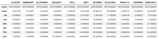
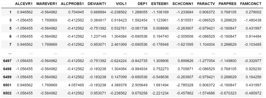
To apply clustering, we need to set the data in similar ranges

clustervar=cluster.copy() clustervar['ALCEVR1']=preprocessing.scale(clustervar['ALCEVR1'].astype('float64')) clustervar['ALCPROBS1']=preprocessing.scale(clustervar['ALCPROBS1'].astype('float64')) clustervar['MAREVER1']=preprocessing.scale(clustervar['MAREVER1'].astype('float64')) clustervar['DEP1']=preprocessing.scale(clustervar['DEP1'].astype('float64')) clustervar['ESTEEM1']=preprocessing.scale(clustervar['ESTEEM1'].astype('float64')) clustervar['VIOL1']=preprocessing.scale(clustervar['VIOL1'].astype('float64')) clustervar['DEVIANT1']=preprocessing.scale(clustervar['DEVIANT1'].astype('float64')) clustervar['FAMCONCT']=preprocessing.scale(clustervar['FAMCONCT'].astype('float64')) clustervar['SCHCONN1']=preprocessing.scale(clustervar['SCHCONN1'].astype('float64')) clustervar['PARACTV']=preprocessing.scale(clustervar['PARACTV'].astype('float64')) clustervar['PARPRES']=preprocessing.scale(clustervar['PARPRES'].astype('float64'))

clustervar

Now we can apply clustering, but before that, we need to know how many clusters would be the optimal. For that, we going to use the elbow method to graph the disantance means of each cluster

clus_train, clus_test = train_test_split(clustervar, test_size=.3, random_state=123)

from scipy.spatial.distance import cdist clusters=range(1,10) meandist=[]

for k in clusters: model=KMeans(n_clusters=k) model.fit(clus_train) clusassign=model.predict(clus_train) meandist.append(sum(np.min(cdist(clus_train, model.cluster_centers_, 'euclidean'), axis=1)) / clus_train.shape[0])

plt.plot(clusters, meandist) plt.xlabel('Number of clusters') plt.ylabel('Average distance') plt.title('Selecting k with the Elbow Method')

model3=KMeans(n_clusters=3) model3.fit(clus_train) clusassign=model3.predict(clus_train)

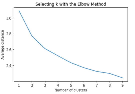
The elbow method suggest 2 or 3 clusters according to the graph

To plot the clusters, we need to reduce the variables, hence we transform the current variables into a canonical variables

from sklearn.decomposition import PCA pca_2 = PCA(2) plot_columns = pca_2.fit_transform(clus_train) plt.scatter(x=plot_columns[:,0], y=plot_columns[:,1], c=model3.labels_,) plt.xlabel('Canonical variable 1') plt.ylabel('Canonical variable 2') plt.title('Scatterplot of Canonical Variables for 3 Clusters') plt.show()

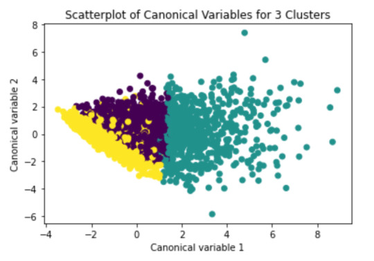
We can see a strong correlation between 2 clusters (Yellow & Purple)

Finally we group the clusters to evaluate the created model

clus_train.reset_index(level=0, inplace=True)

cluslist=list(clus_train['index'])

labels=list(model3.labels_)

newlist=dict(zip(cluslist, labels)) newlist

newclus=DataFrame.from_dict(newlist, orient='index') newclus

newclus.columns = ['cluster']

newclus.reset_index(level=0, inplace=True)

merged_train=pd.merge(clus_train, newclus, on='index') merged_train.head(n=100)

merged_train.cluster.value_counts()

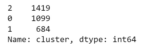
This shows the elements by cluster

clustergrp = merged_train.groupby('cluster').mean() print ("Clustering variable means by cluster") print(clustergrp)

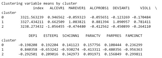
As we can see, Cluster 1 is strong in Marever 1 (use of marijuana) and Alcprobs1 (use of alcohol), on the other hand, cluster 2 is strong in Schconn (school connectedness) and Esteem1 (self esteem).

We can evaluate the relation between clusters

gpa_data=data_clean['GPA1']

gpa_train, gpa_test = train_test_split(gpa_data, test_size=.3, random_state=123) gpa_train1=pd.DataFrame(gpa_train) gpa_train1.reset_index(level=0, inplace=True) merged_train_all=pd.merge(gpa_train1, merged_train, on='index') sub1 = merged_train_all[['GPA1', 'cluster']].dropna()

import statsmodels.formula.api as smf import statsmodels.stats.multicomp as multi

gpamod = smf.ols(formula='GPA1 ~ C(cluster)', data=sub1).fit() print (gpamod.summary())

print ('means for GPA by cluster') m1= sub1.groupby('cluster').mean() print (m1)

print ('standard deviations for GPA by cluster') m2= sub1.groupby('cluster').std() print (m2)

mc1 = multi.MultiComparison(sub1['GPA1'], sub1['cluster']) res1 = mc1.tukeyhsd() print(res1.summary())

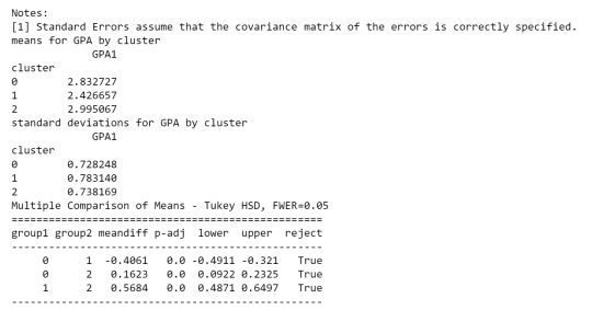
As we can see, the first table shows us data regarding the relationship between each cluster, which indicates that there is a considerable difference.

in the second table, we can see de GPA (Grade Point Average) is higher in cluster 2 where the features related to positive aspects regarding the use of alcohol and marijuana

[practicascfmm]

Lasso Regression

We are running a lasso regression to get the goal is to identify a smaller subset of these predictors that most accurately predicts school connectedness

First, we need to import the necessary libraries and modify the data in order to applying the algoritm.

mport pandas as pd import numpy as np import matplotlib.pylab as plt from sklearn.model_selection import train_test_split from sklearn.linear_model import LassoLarsCV

data = pd.read_csv("tree_addhealth.csv")

data.columns = map(str.upper, data.columns)

data_clean = data.dropna() recode1 = {1:1, 2:0} data_clean['MALE']= data_clean['BIO_SEX'].map(recode1)

predvar= data_clean[['MALE','HISPANIC','WHITE','BLACK','NAMERICAN','ASIAN', 'AGE','ALCEVR1','ALCPROBS1','MAREVER1','COCEVER1','INHEVER1','CIGAVAIL','DEP1', 'ESTEEM1','VIOL1','PASSIST','DEVIANT1','GPA1','EXPEL1','FAMCONCT','PARACTV', 'PARPRES']]

target = data_clean.SCHCONN1

predictors=predvar.copy() from sklearn import preprocessing predictors['MALE']=preprocessing.scale(predictors['MALE'].astype('float64')) predictors['HISPANIC']=preprocessing.scale(predictors['HISPANIC'].astype('float64')) predictors['WHITE']=preprocessing.scale(predictors['WHITE'].astype('float64')) predictors['NAMERICAN']=preprocessing.scale(predictors['NAMERICAN'].astype('float64')) predictors['ASIAN']=preprocessing.scale(predictors['ASIAN'].astype('float64')) predictors['AGE']=preprocessing.scale(predictors['AGE'].astype('float64')) predictors['ALCEVR1']=preprocessing.scale(predictors['ALCEVR1'].astype('float64')) predictors['ALCPROBS1']=preprocessing.scale(predictors['ALCPROBS1'].astype('float64')) predictors['MAREVER1']=preprocessing.scale(predictors['MAREVER1'].astype('float64')) predictors['COCEVER1']=preprocessing.scale(predictors['COCEVER1'].astype('float64')) predictors['INHEVER1']=preprocessing.scale(predictors['INHEVER1'].astype('float64')) predictors['CIGAVAIL']=preprocessing.scale(predictors['CIGAVAIL'].astype('float64')) predictors['DEP1']=preprocessing.scale(predictors['DEP1'].astype('float64')) predictors['ESTEEM1']=preprocessing.scale(predictors['ESTEEM1'].astype('float64')) predictors['VIOL1']=preprocessing.scale(predictors['VIOL1'].astype('float64')) predictors['PASSIST']=preprocessing.scale(predictors['PASSIST'].astype('float64')) predictors['DEVIANT1']=preprocessing.scale(predictors['DEVIANT1'].astype('float64')) predictors['GPA1']=preprocessing.scale(predictors['GPA1'].astype('float64')) predictors['EXPEL1']=preprocessing.scale(predictors['EXPEL1'].astype('float64')) predictors['FAMCONCT']=preprocessing.scale(predictors['FAMCONCT'].astype('float64')) predictors['PARACTV']=preprocessing.scale(predictors['PARACTV'].astype('float64')) predictors['PARPRES']=preprocessing.scale(predictors['PARPRES'].astype('float64'))

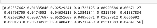
Once we treated the variables, we detect which one has the highest correlation with the response variable and those that will be exculded from the algoritm, in this case those that show zeros.

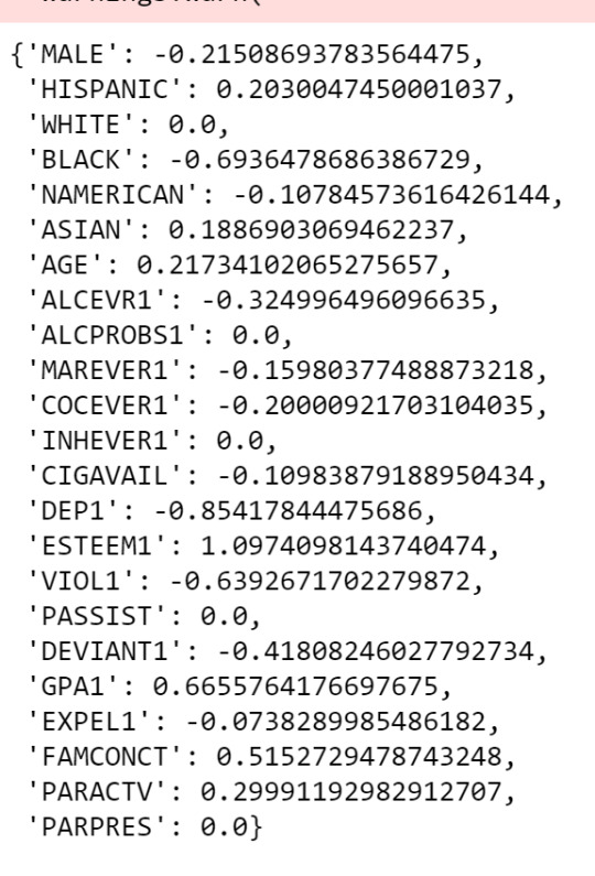
Variables like "White", "Black" & "AlcProbs1" will be excluded, while variables as "Esteem1" & "Dep1" have the highest correlation whit the response variable (positively & negatively, respecively). We can see the same data on this plot:

m_log_alphas = -np.log10(model.alphas_) ax = plt.gca() plt.plot(m_log_alphas, model.coef_path_.T) plt.axvline(-np.log10(model.alpha_), linestyle='--', color='k', label='alpha CV') plt.ylabel('Regression Coefficients') plt.xlabel('-log(alpha)') plt.title('Regression Coefficients Progression for Lasso Paths')

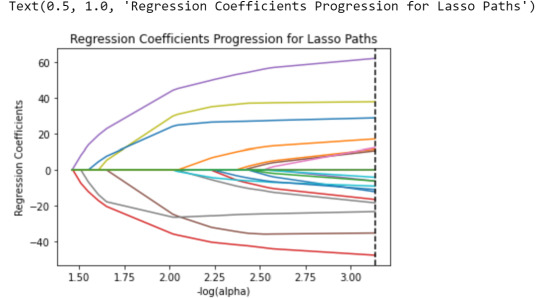
The lines represent the regression coefficients that we saw above.

Finally, we apply MSE & R-squre to evaluate the model

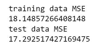
from sklearn.metrics import mean_squared_error train_error = mean_squared_error(tar_train, model.predict(pred_train)) test_error = mean_squared_error(tar_test, model.predict(pred_test)) print ('training data MSE') print(train_error) print ('test data MSE') print(test_error)

rsquared_train=model.score(pred_train,tar_train) rsquared_test=model.score(pred_test,tar_test) print ('training data R-square') print(rsquared_train) print ('test data R-square') print(rsquared_test)

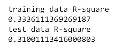
In both cases, both MSE and R-Square the results don't differ so much between the training & testing set.

[practicascfmm]

Random Forrest

Running a Random Forrest in Python

from pandas import Series, DataFrame import pandas as pd import numpy as np import os import matplotlib.pylab as plt from sklearn.model_selection import train_test_split from sklearn.tree import DecisionTreeClassifier from sklearn.metrics import classification_report import sklearn.metrics # Feature Importance from sklearn import datasets from sklearn.ensemble import ExtraTreesClassifier

AH_data = pd.read_csv("tree_addhealth.csv") data_clean = AH_data.dropna()

data_clean.dtypes data_clean.describe()

predictors = data_clean[['BIO_SEX','HISPANIC','WHITE','BLACK','NAMERICAN','ASIAN','age', 'ALCEVR1','ALCPROBS1','marever1','cocever1','inhever1','cigavail','DEP1','ESTEEM1','VIOL1', 'PASSIST','DEVIANT1','SCHCONN1','GPA1','EXPEL1','FAMCONCT','PARACTV','PARPRES']]

targets = data_clean.TREG1

pred_train, pred_test, tar_train, tar_test = train_test_split(predictors, targets, test_size=.4)

pred_train.shape pred_test.shape tar_train.shape tar_test.shape

Build model on training data

from sklearn.ensemble import RandomForestClassifier

classifier=RandomForestClassifier(n_estimators=25) classifier=classifier.fit(pred_train,tar_train)

predictions=classifier.predict(pred_test)

sklearn.metrics.confusion_matrix(tar_test,predictions) sklearn.metrics.accuracy_score(tar_test, predictions)

fit an Extra Trees model to the data

model = ExtraTreesClassifier() model.fit(pred_train,tar_train)

display the relative importance of each attribute

print(model.feature_importances_)

##Given that the Random Forrest doesn't show a tree decision, we get the wheight of each variable with the script above. It appears in the same order that we put in the features chain.

So, we can see that 'marever1' (marihuana consumption) is the feature that it has te biggest weight, followed by 'GPA1' (grade point average).

Accurancy Script:

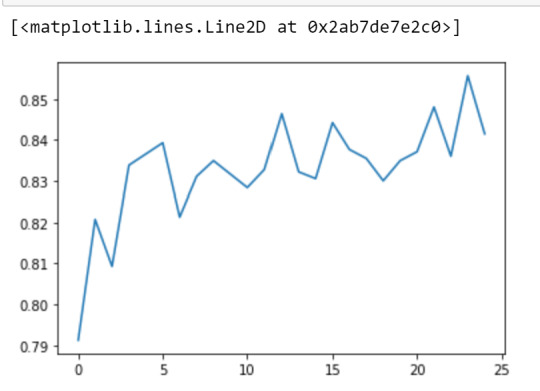
""" Running a different number of trees and see the effect of that on the accuracy of the prediction """

trees=range(25) accuracy=np.zeros(25)

for idx in range(len(trees)): classifier=RandomForestClassifier(n_estimators=idx + 1) classifier=classifier.fit(pred_train,tar_train) predictions=classifier.predict(pred_test) accuracy[idx]=sklearn.metrics.accuracy_score(tar_test, predictions)

plt.cla() plt.plot(trees, accuracy)

[practicascfmm]

Decision Tree -Regresion-

ACHIVEMENT:

Make a prediction of the lower price of a house according to its characteristics an enviroment

VARIABLES / FEATURES:

CRIM: per capita crime rate by town

ZN: proportion of residential land zoned for lots over 25,000 sq.ft.

INDUS: proportion of non-retail business acres per town

CHAS: Charles River dummy variable (= 1 if tract bounds river; 0 otherwise)

NOX: nitric oxides concentration (parts per 10 million)

RM: average number of rooms per dwelling

AGE: proportion of owner-occupied units built prior to 1940

DIS: weighted distances to five Boston employment centres

RAD: index of accessibility to radial highways

TAX: full-value property-tax rate per $10,000

PTRATIO: pupil-teacher ratio by town

B: 1000(Bk - 0.63)^2 where Bk is the proportion of blacks by town

LSTAT: % lower status of the population

MEDV: Median value of owner-occupied homes in $1000's

import numpy as np import pandas as pd

import matplotlib.pyplot as plt

from sklearn.datasets import load_boston from sklearn.model_selection import train_test_split from sklearn.tree import DecisionTreeRegressor from sklearn.tree import plot_tree from sklearn.tree import export_graphviz from sklearn.tree import export_text from sklearn.model_selection import GridSearchCV from sklearn.metrics import mean_squared_error

import warnings warnings.filterwarnings('once')

boston = load_boston(return_X_y=False) datos = np.column_stack((boston.data, boston.target)) datos = pd.DataFrame(datos,columns = np.append(boston.feature_names, "MEDV")) datos.head(3)

X_train, X_test, y_train, y_test = train_test_split( datos.drop(columns = "MEDV"), datos['MEDV'], random_state = 123 )

modelo = DecisionTreeRegressor( max_depth = 3, random_state = 123 )

modelo.fit(X_train, y_train)

fig, ax = plt.subplots(figsize=(12, 5))

print(f"Profundidad del árbol: {modelo.get_depth()}") print(f"Número de nodos terminales: {modelo.get_n_leaves()}")

plot = plot_tree( decision_tree = modelo, feature_names = datos.drop(columns = "MEDV").columns, class_names = 'MEDV', filled = True, impurity = False, fontsize = 10, precision = 2, ax = ax )

This decision tree suggest that a house with a average number of rooms per dwelling <6.9 and % lower status of the population > 14.39 and a per capita crime rate by town > 6.99 has the lower price (11.58)