rfmdataanalysis

[rfmdataanalysis]

National Champion 2023, Go Blue.

[rfmdataanalysis]

RIP Charlie Munger.

[rfmdataanalysis]

SAS Cortex Analytics Simulation

A Simulation Game for Customer Retention Scenario

Game Description

Telc, a telecom company specialized in mobile communications, is turning 10 years (120 months). After their initial big splash, they have grown steadily, welcoming about 3% more clients every year. Shareholders are satisfied with this performance considering that telecom is a very competitive market where clients are constantly looking for a better deal. To celebrate its 10-year anniversary, Telc is planning an innovative marketing campaign to reward their clients and increase their loyalty.

Over the last six months, the Marketing and Business Intelligence department has been planning an entertainment event where some subscribers are invited to a 4-course dinner with live music performed by a local talent.

The main objective is to make the clients more loyal by developing a sense of belonging to the company. By inviting those who are more likely to leave, the company wishes to prevent the churn and to increase loyalty. It has been decided that if a client gets invited to the dinner, all family members from the same household who are Telc clients get invited to the same dinner. The database of Telc identifies which clients are in the same family.

A year ago, a pilot study was carried out to assess the effect of a similar event (i.e., dinner campaign) targeting 5% of their customers chosen at random. These customers are identified by the variable promo =’True’. We are now twelve months away from the pilot project. It is therefore possible to know who left in this time window. The pilot study was useful as a benchmark in determining the cost of organizing dinner events. The costs have been broken down by invitation, whether the invited client goes to the event or not. The costs are described below:

• $10 per invitation (i.e., guest) for the food and drink, • $10,000 per 5,000 invitations (i.e., guests) for the fixed costs (renting room and sound system, paying the artist, etc.)

Even when clients are not able to make it to the event, getting an invitation may have a positive effect. Customers cannot be forced to attend the dinner and the company can only decide to invite them or not. Therefore, it makes sense to measure the effect of the marketing campaign.

Your Task and Performance You will be given some information (e.g., behavioral, demographic, historical) about the current Telc subscribers (refer to the variable description table at the end of this document). You must decide which families and how many families to invite to the dinner. You will submit your decision through the game leaderboard that will give you immediate feedback on your performance.

Telc is constantly evaluating its plans to keep a 50% profit margin on the monthly plan rates. Therefore, the profit generated by one client is 50% of their plans cost in the next 24 months, or until they leave.

This is a business simulation in which customers’ behavior is simulated and known in advance. As a result, the effect of the marketing campaign (i.e., decision to invite or not) on the behavior of the clients in the next two years can be assessed.

Your performance will be based on the total profit generated in 24 months, minus the total cost of the event based on the number of invitations. With a good retention strategy, you should do better than the baseline, which is not inviting any clients to the event or not organizing the event (i.e., additional profit of $0).

Data and Timeline To better clarify the context, the timeline is presented below: • Telc was founded 10 years ago, the first clients arrived at time T = 1 month • We are now at time 120: T = 120 months • A pilot study was carried out at time T = 108 months using the available information of all the clients in this period of time • The file train.sas7bdat contains information on all the clients at time 108: – The same file includes the variable “churn_in_12” that indicates whether or not the client left between time 108 and 120 • The file score.sas7bdat contains information on all the clients at time 120: – Clients who left between times 108 and 120 are not in the file, but new clients are there. • The online platform knows how much profit is made by all clients in the next 24 months or T = 144, if you invite them, and if you do not invite them. • Your performance is based on the Net Profit, which equals total amount of profit

How to Play the Game This game is designed to be played in 2 rounds. The costs presented in both rounds remain the same. Please review each section below carefully for more details.

Round 1: Targeting churning customers without the pilot

IMPORTANT: For round 1, you need to make a decision without using the information obtained by the pilot. This means that you must only use the clients with promo=”False” in your analysis. You can use the filter node to exclude the clients based on their ‘promo’ attributes. Multiple strategies can support the business problem reasonably well and therefore you are expected to come up with your own approach to address the business problem.

Round 2: Using the information obtained from the pilot

In round 2, you may use all the data. Information from the pilot study may help you target clients even more efficiently, possibly leading to a better solution than in round 1. This means that you do not need to filter and exclude any clients – i.e., you can use both the clients with promo=”False” and promo=”True” in your analysis.

How to Submit a Decision for Each Round You must decide which families and how many families to invite. You need to prepare a csv file with only one column: unique_family. Please note that this variable is a unique identifier of a family that you want to invite. This variable is only shown in the score dataset: score.sas7bdat You will have to upload your csv file to the game leaderboard (the link will be provided to you). The cost of the invitations will be automatically calculated, and the net profit (company’s profit minus the campaign cost) and the players rankings will be immediately shown in the leaderboard. The game leaderboard allows for multiple uploads (a total of 70 uploads per round) and will provide immediate feedback. Therefore, if you are not happy with your results and ranking, you can change your strategy and test other models and upload another csv file to the leaderboard.

A Note for SAS Viya Users If you are playing this game on SAS Visual Data Mining and Machine Learning (SAS Viya), the train (train.sas7bdat) and score (score.sas7bdat) datasets are uploaded on the Viya system for you. Upon your log-on to the system and opening your game project, you will have access to the train dataset and its variables to train your models. After training your models, you will then access the score dataset to score your data and visualize your results. All the steps and instructions are provided in the material accompanying the game for Viya.  

Figures and Tables The figure below demonstrates the business context, the available information and your role as the Customer Relationship Manager who is helping the company with its marketing campaign:

In order to play the game and make decisions, you will have access to a dataset of around 1 million subscribers. The variables of the dataset and their descriptions are listed below:

I am the 2nd place winner of Wells Fargo Cortex Analytics Simulation Challenge

[rfmdataanalysis]

SAS Macro and Proc SQL Examples

/* Example: select distinct car type into a list */

Proc sql noprint;    select distinct type into :list separated by “ “

   from sashelp.cars;

quit;

%put ERROR- &list  /* print output list in color red */;

/* Example: select distinct car type into a list 2 */

%macro charlist (var=, dsn=);

%global list /* define global table list */;

Proc sql noprint;   select distinct &var into :list separated by “ “

  from &dsn;

quit;

%mend charlist;

%charlist(var=make, dsn=sashelp.cars) %put &list;

%charlist(var=species, dsn=sashelp.fish) %put &list; 

%charlist(var=age, dsn=sashelp.class) %put &list

Proc sql noprint;   select distinct type into :list separated by “ “

  from sashelp.cars;

quit;

%put ERROR- &list  /* print output list in color red */;

/* Example: macro carfinder */

options mcompilenote=noautocall;

%macro carfinder (car);

proc sql;

   tittle1 “&car”;

  select model, type, msrp

   from sashelp.cars

   where upcase(make)=%upcase(”&car.”))

   order by 1;

quit;

%mend carfinder;

%carfinder(bmw);

/* Example: macro carfinder 2 */

options mcompilenote=noautocall;

%macro carfinder (car);

proc sql noprint;

   select mean(msrp) format=dollar7. into :mean_msrp

   from sashelp.cars

   where make=&car;

reset print;

  tittle1 “&car”;

  title2 “Average MSRP: mean_msrp”;

  footnote “&car”;

 select model, type, msrp

  from sashelp.cars

  where upcase(make)=%upcase(”&car.”))

  order by model;

quit;

%mend carfinder;

%carfinder(chevrolet);

/* Example: macro carcheck using macros created above */

%macro carcheck(car);

%charlist(var=make, dsn=sashelp.cars)

 %if &car in &list %then %do;

       %charlist(var=type, dsn=sashelp.cars)

       %carfinder(&car)

  %end;

%else %do;

%put ERROR No &car.s;

%put NOTE: Cars include &list..;

%mend carcheck;

%carcheck(Chevrolet)

%carcheck(Chevy)

/* Example: macro deleteAll , use as cleaning utility macro*/

/* WINDOW Environment */

%marco deleteAll;

options nonotes;

%local vars;

proc sql noteprint;

select name into: vars separate by ‘ ‘

from dictionary.macro

where scope=‘GLOBAL’ and name not like ‘SYS%’ and name not like ‘SQL%’;

quit;

%symdel &vars;

options notes;

%put NOTE: &sqlobs macro variable(s) deleted.;

%mend deleteAll;

%deleteall

%put _user_;

/* List Dictionary tables, columns, macros */

options nolabel;

proc sql;

select * from dictionary.tables

   where libname=‘SASHELP’;

select * from dictionary.columns

   where libname=‘SASHELP’;

select * from dictionary.macros

  where libname=‘SASHELP’;

quit;

/* Examplle: marco deleall 2  Studio and Enterprise Guide*/

%macro deleteAll;

options nonotes;

%local vars;

proc sql noprint;

select name into: vars separated by ‘ ‘

  from dictionay.macros

  where scope=‘GLOBAL’

and  and name not like ‘SYS%’ and name not like ‘SQL%’

and  and name not like ‘STUDIO%’ and name not like ‘CLIENT%’

and  and name not like ‘GRAPH%’ and name not like ‘OLD%’

and  and name not like ‘SAS%’ and name not like ‘USER%’

and  and name not like ‘/_%’ escape ’ /’;

%symdel &vars; options notes;

%put NOTE: &sqlobs macro variable(s) deleted;

%mdeleteALL;

%global x y z /* create dummy global vars to test macro */;

%deleteall

Reference:

John McCall SAS Tutorial | Getting the Most out of SAS Macro and SQL on YouTube

[rfmdataanalysis]

SAS Visual Analytics Basics

Start SAS Visual Analytics If you are using another SAS application (for example, SAS Drive), you can access SAS Visual Analytics from the side menu. Click “Hamburger” icon in the upper left of the page, and then click Explore and Visualize. Here is an example of what you might see in the side menu:

The SAS Visual Analytics Interface In SAS Visual Analytics, you can design reports, view reports and explore data. You can run interactive, predictive models if SAS Visual Statistics and SAS Visual Data Mining and Machine Learningare licensed at your site.

Here are the features of the interface:

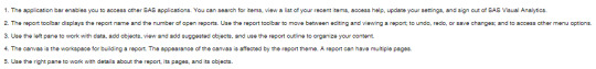
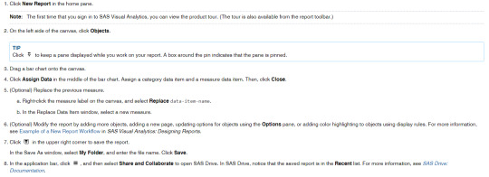
Create a Report

Steps  to edit reports in SAS Visual Analytics.

View a Report

You can view reports in SAS Visual Analytics or by using one of the SAS Visual Analytics Apps. Here are ways to view a report:

Data Tasks In general, data-related tasks are initiated from the left panes.

Object Tasks Here are other common tasks that can be completed using other panes on the left side or menus in the user interface

Reference:

https://documentation.sas.com/doc/en/vacdc/8.5/vareportsgs/p1picx03kj4o4qn1rfcaewemz50g.htm

[rfmdataanalysis]

Data Quality Operations

Identification Analysis

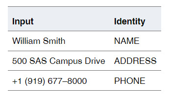
To take advantage of the value of your data, you need to know the types of data that you have. Identification Analysis helps you understand your data by naming the type of the content in each variable. Identifying your data enables data profiling, data preparation, data cleansing, and data analysis.

Identification Analysis generates text classifications; it does not determine the database data type of your data, such as CHAR, BOOLEAN, or INTEGER. Instead, Identification Analysis reads text values and determines the semantic type of those values.

The output of Identification Analysis is a named classification that is known as an identity. The following example shows how identities are derived from text values:

Gender Analysis

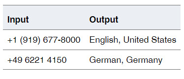
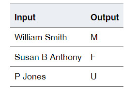
When your data represents individual persons, you can analyze that data to determine the gender of each person. Gender data can be useful in subsequent statistical analysis, particularly in the domains of medical reporting and product marketing.

The input for Gender Analysis is a text string, and the output is gender code, as shown in the following example:

Parsing Parsing breaks a text string into a set of constituent sub-strings. The sub-strings represent a set of semantically atomic portions of the original string. In other words, each of the outputs has meaning in its own right.

For example, consider the sub-strings that can make up a person’s name. Most names contain a given name and a family name. A given name and a family name both have meaning of their own. You can use a Parsing operation to generate separate instances of the given name and family name:

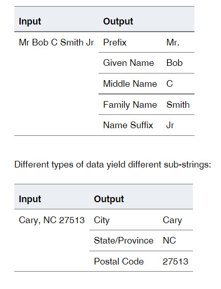
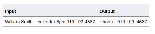
Extraction Sometimes, even in relational data, you can have text strings with little or no structure. It might not always be possible to parse such strings into constituent components. Instead, you might want to simply scan the string and extract a few meaningful attributes. An example of such an Extraction operation is as follows:

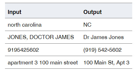
Standardization Standardization transforms text strings by rendering them in a preferred format. A Standardization operation can rearrange words, change individual words or symbols, and apply casing rules.

Matching

Matching operations provide a way to apply fuzzy matching logic in various data cleansing and data integration operations. You can use fuzzy matching logic to find and remove duplicate records, implement fuzzy searches, perform fuzzy joins, and more.

Matching operations are based on the generation of text strings called matchcodes. A matchcode is a fuzzy representation of an input text string. If two or more text strings yield the same matchcode, then those strings match. For example, the following records constitute a match:

You perform fuzzy matching operations by generating matchcodes for your data and then sorting and comparing the matchcodes, or using them as criteria for joins or other data integration operations.

Reference:

https://documentation.sas.com/doc/en/dqcdc/3.5/dqgs/p04xj2uanyz22wn1mnyv7if0924n.htm

[rfmdataanalysis]

SAS Macro Examples

*Example: Import All CSV Files That Exist within a Directory;

%macro drive(dir,ext); 

   %local cnt filrf rc did memcnt name;

   %let cnt=0;

   %let filrf=mydir;

   %let rc=%sysfunc(filename(filrf,&dir));

   %let did=%sysfunc(dopen(&filrf));

   %if &did ne 0 %then %do;

      %let memcnt=%sysfunc(dnum(&did));

      %do i=1 %to &memcnt;

         %let name=%qscan(%qsysfunc(dread(&did,&i)),-1,.);

         %if %qupcase(%qsysfunc(dread(&did,&i))) ne %qupcase(&name) %then %do;

            %if %superq(ext) = %superq(name) %then %do;

               %let cnt=%eval(&cnt+1);

               %put %qsysfunc(dread(&did,&i));

               proc import datafile="&dir\%qsysfunc(dread(&did,&i))" out=dsn&cnt 

                  dbms=csv replace;

               run;

            %end;

         %end;

       %end;

    %end;

  %else %put &dir cannot be opened.;

  %let rc=%sysfunc(dclose(&did));

%mend drive;

%drive(c:\temp,csv)

/* Example: List All Files within a Directory Including Subdirectories */

/*  This macro currently works for Windows platforms, but could be modified for  other operating environments. */

/* This example will not run if you use the LOCKDOWN system option. */

%macro list_files(dir,ext);  %local filrf rc did memcnt name i;  %let rc=%sysfunc(filename(filrf,&dir));  %let did=%sysfunc(dopen(&filrf));      

  %if &did eq 0 %then %do;    %put Directory &dir cannot be open or does not exist;    %return;  %end;

  %do i = 1 %to %sysfunc(dnum(&did));  

  %let name=%qsysfunc(dread(&did,&i));

     %if %qupcase(%qscan(&name,-1,.)) = %upcase(&ext) %then %do;        %put &dir\&name;      %end;      %else %if %qscan(&name,2,.) = %then %do;                %list_files(&dir\&name,&ext)      %end;

  %end;   %let rc=%sysfunc(dclose(&did));   %let rc=%sysfunc(filename(filrf));    

%mend list_files; %list_files(c:\temp,sas)

/* Example: Place All SAS Data Set Variables into a Macro Variable */

data one;  input x y; datalines; 1 2 ;

%macro lst(dsn);  %local dsid cnt rc;  %global x;  %let x=;  %let dsid=%sysfunc(open(&dsn));   %if &dsid ne 0 %then %do;  %let cnt=%sysfunc(attrn(&dsid,nvars));

  %do i = 1 %to &cnt;    %let x=&x %sysfunc(varname(&dsid,&i));   %end;

 %end;    %else %put &dsn cannot be open.;  %let rc=%sysfunc(close(&dsid));

%mend lst;

%lst(one)

%put macro variable x = &x;  

*Example: Using a Macro to Create New Variable Names from Variable Values;

data teams;  input color $15. @16 team_name $15. @32 game1 game2 game3; datalines; Green          Crickets        10 7 8 Blue           Sea Otters      10 6 7 Yellow         Stingers        9 10 9 Red            Hot Ants        8 9 9 Purple         Cats            9 9 9 ;

%macro newvars(dsn);

data _null_;  set &dsn end=end;  count+1;  call symputx('macvar'||left(count),compress(color)||compress(team_name)||"Total");  if end then call symputx('max',count); run;

data teamscores;  set &dsn end=end;

%do i = 1 %to &max;  if _n_=&i then do;    &&macvar&i=sum(of game1-game3);    retain &&macvar&i;    keep &&macvar&i;  end; %end; if end then output;

%mend newvars;

%newvars(teams)

proc print noobs;  title "League Team Game Totals"; run;  

/*Example : Create a Quoted List Separated by Spaces*/

data one; input empl $; datalines; 12345 67890 45678 ;

%let list=; data _null_; set one;       call symputx('mac',quote(strip(empl)));   call execute('%let list=&list &mac'); run;

%put &=list;

/*Example: Retrieve Each Word from a Macro Variable List */

%let varlist = Age Height Name Sex Weight;

%macro rename;   %let word_cnt=%sysfunc(countw(&varlist));   %do i = 1 %to &word_cnt;     %let temp=%qscan(%bquote(&varlist),&i);     &temp = _&temp   %end; %mend rename;

data new;   set sashelp.class(rename=(%unquote(%rename))); run;

proc print; run;

/*Example: Dynamically Determine the Number of Observations and Variables in a SAS Data Set */

data test;   input a b c $ d $;   datalines; 1 2 A B 3 4 C D ;

%macro obsnvars(ds);   %global dset nvars nobs;   %let dset=&ds;   %let dsid = %sysfunc(open(&dset));

  %if &dsid %then %do;      %let nobs =%sysfunc(attrn(&dsid,nlobs));      %let nvars=%sysfunc(attrn(&dsid,nvars));      %let rc = %sysfunc(close(&dsid));   %end;

  %else %put open for data set &dset failed - %sysfunc(sysmsg()); %mend obsnvars;

%obsnvars(test)

%put &dset has &nvars variable(s) and &nobs observation(s).;

/*Example: Loop through Dates Using a Macro %DO Loop*/

%macro date_loop(start,end);   %let start=%sysfunc(inputn(&start,anydtdte9.));   %let end=%sysfunc(inputn(&end,anydtdte9.));   %let dif=%sysfunc(intck(month,&start,&end));     %do i=0 %to &dif;      %let date=%sysfunc(intnx(month,&start,&i,b),date9.);      %put &date;     %end;   %mend date_loop;

  %date_loop(01jul2015,01feb2016)

/*Example A: This example enables you to step through only the characters that are passed to the macro as a parameter to the macro variable named &LST.*/

%macro iterm(lst); %let finish=%sysfunc(countw(&lst));  %do i = 1 %to &finish;   %put %scan(&lst,&i);  %end; %mend iterm;

%iterm(a c e)

/*Example B: This example enables you to step through the characters between the &BEG and &END values. */

%macro iterm(beg,end); %do i = %sysfunc(rank(&beg)) %to %sysfunc(rank(&end));  %put %sysfunc(byte(&i)); %end; %mend iterm;

%iterm(a,e)

/*Example: Retrieve the File Size, Create Time, and Last Modified Date of an External File*/

%macro FileAttribs(filename);            %local rc fid fidc Bytes CreateDT ModifyDT;  %let rc=%sysfunc(filename(onefile,&filename));  %let fid=%sysfunc(fopen(&onefile));     %if &fid ne 0 %then %do;    %let Bytes=%sysfunc(finfo(&fid,File Size (bytes)));    %let CreateDT=%sysfunc(finfo(&fid,Create Time));      %let ModifyDT=%sysfunc(finfo(&fid,Last Modified));      %let fidc=%sysfunc(fclose(&fid));      %let rc=%sysfunc(filename(onefile));  %put NOTE: File size of &filename is &bytes bytes;      %put NOTE- Created &createdt;        %put NOTE- Last modified &modifydt;     %end;        %else %put &filename could not be open.; %mend FileAttribs;

%FileAttribs(c:\aaa.txt)

Reference:

https://documentation.sas.com/doc/en/pgmsascdc/9.4_3.5/mcrolref/n0ctmldxf23ixtn1kqsoh5bsgmg8.htm

[rfmdataanalysis]

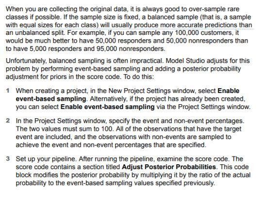
Adjust Posterior Probabilities for Event-based Sampling

When you create a SAS® Visual Data Mining and Machine Learning project where event-based sampling is enabled, the posterior probabilities are adjusted for the prior probabilities (priors) in the score code of a modeling node.

To determine whether the priors are used, examine the code in the Node Score Code of the node results. If priors are used, then the score code should adjust the posterior probabilities like in the example below. Note that 0.8005033557 represents the prior when the target level is 0, and 0.1994966443 represents the prior when the target level is 1.

 Note: 1- 0.1994966443 =  0.8005033557.

* Adjust Posterior Probabilities for 10% Event and 90% Non-Event ;

* If P is blank, use event and non-event percent;

IF ‘P_TARGET_BINARY1′= . THEN  ‘P_TARGET_BINARY1′=0.1;

IF ‘P_TARGET_BINARY0′= . THEN  ‘P_TARGET_BINARY0′=0.9;

'P_TARGET_BINARY0′ = 'P_TARGET_BINARY0′ * 0.8005033557/0.9;

'P_TARGET_BINARY1′ = 'P_TARGET_BINARY1′ * 0.1994966443/0.1;

Reference:

https://support.sas.com/kb/67/609.html

[rfmdataanalysis]

[rfmdataanalysis]

RFM Data Analysis and Machine Learning turned 6 today!

[rfmdataanalysis]

SAS CAUSALTRT Procedure Overview

The CAUSALTRT procedure estimates the average causal effect of a binary treatment, T, on a continuous or discrete outcome, Y. Although the causal effect that is defined and estimated in PROC CAUSALTRT is called a treatment effect, it is not confined to effects that result from controllable treatments (such as effects in an experiment). Depending on the application, the binary treatment variable T can represent an intervention (such as smoking cessation versus control), an exposure to a condition (such as attending a private versus public school), or an existing characteristic of subjects (such as high versus low socioeconomic status). The CAUSALTRT procedure can estimate two types of causal effects: the average treatment effect (ATE) and the average treatment effect for the treated (ATT). 

The CAUSALTRT procedure implements causal inference methods that are designed primarily for use with data from nonrandomized trials or observational studies. In an observational study, you observe the treatment T and the outcome Y without assigning subjects randomly to the treatment conditions. Instead, subjects "select" themselves into the treatment conditions according to their pretreatment characteristics. If these pretreatment characteristics are also associated with the outcome Y, they induce a specious relationship between T and Y and hence cloud the causal interpretation of T on Y. Therefore, estimating the causal effect of T in observational studies usually requires adjustments that remove or counter the specious effects that are induced by the confounding variables.

To adjust for the effects of the confounding variables, you can model either the treatment assignment T or the outcome Y, or both. Modeling the treatment leads to inverse probability weighting methods, and modeling the outcome leads to regression adjustment methods. Combined modeling of the treatment and outcome leads to doubly robust methods that can provide unbiased estimates for the treatment effect even if one of the models is misspecified.

[rfmdataanalysis]

A SAS CAUSALTRT Procedure Example

This example uses data from a hypothetical nonrandomized trial. (Note: For marketing usage, we could replace treatment variable Drug values ‘Drug A’ and ‘Drug X’ with ‘Emailed’ and ‘Holdout’, outcome variable Diabetes with Purchased for the dataset.)

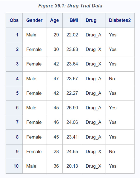
Suppose that 486 patients in a trial are at risk for developing type 2 diabetes and are allowed to choose which of two preventive drugs they want to receive. For this study, the outcome of interest is whether a patient develops type 2 diabetes within five years. The nonrandom assignment of patients to treatment conditions does not control for confounding variables that might explain any observed difference between the treatment conditions. The hypothetical data set Drugs contains the following variables:

Age: age at the start of the trial

BMI: body mass index at the start of the trial

Diabetes2: indicator for whether a patient developed type 2 diabetes, with values Yes and No

Drug: indicator of treatment assignment, with values Drug_A and Drug_X

Gender: gender

The first 10 observations in the Drugs data set are listed in Figure 36.1.

The following statements invoke the CAUSALTRT procedure and request the estimation of the average treatment effect (ATE) by using the inverse probability weighting method with ratio adjustment (METHOD=IPWR):

proc causaltrt data=drugs method=ipwr ppsmodel;   class Gender;   psmodel Drug(ref='Drug_A') = Age Gender BMI;   model Diabetes2(ref='No') / dist = bin; run;

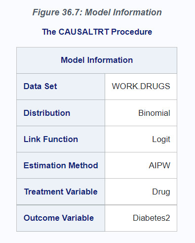
The results of this analysis are shown in the following figures. In Figure 36.2, PROC CAUSALTRT displays information about the estimation method used, the outcome variable, and the treatment variable.

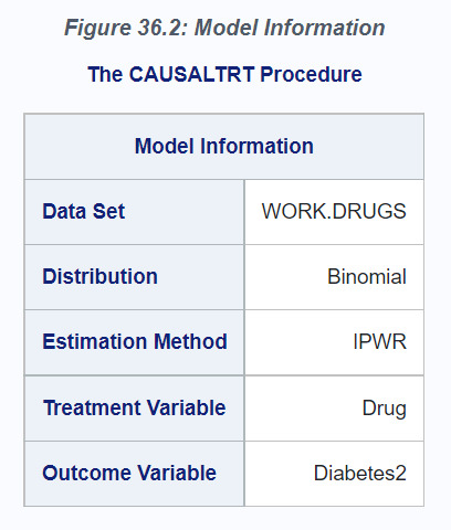
The METHOD= option in the PROC CAUSALTRT statement specifies the estimation method to be used. The outcome variable, Diabetes2, is specified in the MODEL statement, and the treatment variable, Drug, is specified in the PSMODEL statement.

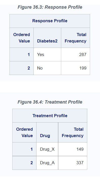
The DIST=BIN option in the MODEL statement identifies the outcome as a binary variable, and the ref='No' option identifies No as the reference level. In the PSMODEL statement, the ref='Drug_A' option identifies Drug_A as the reference (control) condition when the treatment assignment is modeled and the ATE is estimated. The frequencies for the outcome and treatment variable categories are listed in the "Response Profile" (Figure 36.3) and "Treatment Profile" (Figure 36.4) tables, respectively.

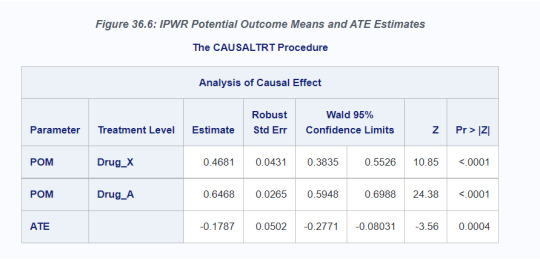
The IPWR estimation method uses inverse probability weighting to estimate the potential outcome means and ATE. The inverse probability weights are estimated by inverting the predicted probability of receiving treatment (that is, the Drug_X condition), which is estimated from a logistic regression model that is specified in the PSMODEL statement. The probability of receiving treatment is called the propensity score, and hence the regression model fit by the PSMODEL statement is also called the propensity score model. In this example, the predictors of the propensity score model are Age, Gender, and BMI. The PPSMODEL option in the PROC CAUSALTRT statement displays the parameter estimates for the propensity score model, as shown in Figure 36.5.

The estimates for the potential outcome means (POM) and ATE are displayed in the "Analysis of Causal Effect" table (Figure 36.6). The ATE estimate of –0.1787 indicates that Drug_X is more effective on average than Drug_A in preventing the development of type 2 diabetes. The ATE is significantly different from 0 at the 0.05 -level, as indicated by the 95% confidence interval (–0.2771, –0.0803) or the p-value (0.0004).

The ATE of Drug_X compared to Drug_A can also be estimated by using augmented inverse probability weights (AIPW). In addition to a propensity score model, the AIPW estimation method incorporates a model for the outcome variable, Diabetes2, into the estimation of the potential outcome means and ATE. The AIPW estimation method is doubly robust and provides unbiased estimates for the ATE even if one of the outcome or treatment models is misspecified.

The following statements invoke the CAUSALTRT procedure and use the AIPW estimation method to estimate the ATE:

proc causaltrt data=drugs method=aipw;   class Gender;   psmodel Drug(ref='Drug_A') = Age Gender BMI;   model Diabetes2(ref='No') = Age Gender BMI / dist = bin; run;

For this example, the same set of effects is specified in both the MODEL and PSMODEL statements, but in general this need not be the case. The use of the AIPW estimation method for this PROC CAUSALTRT step is reflected in the "Model Information" table (Figure 36.7).

As shown in Figure 36.8, the AIPW estimate for the ATE is –0.1709, which is similar to the IPWR estimate of –0.1787. Moreover, the AIPW standard error estimate for ATE is slightly smaller than that of the IPWR. The AIPW 95% confidence interval for ATE is also slightly narrower than that of the IPWR.

Codes for this example:

/*-----------------------------------------------------------------            S A S   S A M P L E   L I B R A R Y                  

     NAME: CTRTGS                                                     TITLE: Getting Started Example for PROC CAUSALTRT               PRODUCT: STAT                                                      SYSTEM: ALL                                                        KEYS: Inverse probability weights                               PROCS: CAUSALTRT                                                  DATA:                                                      

  SUPPORT: milamm   ��                                                   REF: PROC CAUSALTRT, GETTING STARTED EXAMPLE                    MISC:                                                       -----------------------------------------------------------------*/

data drug1;   do jorder=1 to 490;      if (ranuni(99) < .55) then Gender='Male  ';      else                       Gender='Female';

     Age= 30 + 20*ranuni(99) + 3*rannor(9);      if (Age < 25) then  Age= 20 - (Age-25)/2;      Age= int(Age);

     BMI= 20 + 6*ranuni(99) + 0.02*Age + rannor(9);      if (BMI < 18) then BMI= 18 - (BMI-18)/4;      BMI= int(BMI*100) / 100;

     pscore= 4. - 0.25*Age + 0.2*BMI + 0.02*rannor(99);      if (Gender='Female') then pscore= pscore - 0.2;      output;   end; run;

proc sort data=drug1 out=drug2;   by pscore; run; proc rank data=drug2 out=drug3 descending;   var pscore;   ranks porder; run;

data drug4;   set drug3;   if (porder < 150) then do;      if (ranuni(99) < .45) then Drug= 'Drug_X';      else                       Drug= 'Drug_A';   end;   else if (porder < 300) then do;      if (ranuni(99) < .35) then Drug= 'Drug_X';      else                       Drug= 'Drug_A';   end;   else if (porder < 450) then do;      if (ranuni(99) < .25) then Drug= 'Drug_X';      else                       Drug= 'Drug_A';   end;   else                          Drug= 'Drug_A'; run;

data drug5;   set drug4;   if (porder > 4); run;

proc sort data=drug5 out=drugs (keep=Drug Gender Age BMI);   by jorder; run;

data drug6;   set drug5;   pdev = -.1 + .02*age;   if (Drug = 'Drug_X') then pdev = pdev -.2;   if (Gender = 'Male') then pdev = pdev - .1;   psdev = exp(pdev)/(1+exp(pdev));   if (pdev > ranuni(99)) then Diabetes2 = 'Yes';   else                      Diabetes2 = 'No'; run;

proc sort data=drug6 out=drugs (keep=Drug Gender Age BMI Diabetes2);   by jorder; run;

proc print data=drugs(obs=10); run;

proc causaltrt data=drugs method=ipwr ppsmodel;   class Gender;   psmodel Drug(ref='Drug_A') = Age Gender BMI;   model Diabetes2(ref='No') / dist = bin; run;

proc causaltrt data=drugs method=aipw;   class Gender;   psmodel Drug(ref='Drug_A') = Age Gender BMI;   model Diabetes2(ref='No') = Age Gender BMI / dist = bin; run;

Reference

SAS 9.4 and SAS Viya 3.4 Programming Documentation.

[rfmdataanalysis]

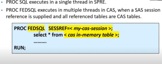
Working with data in SAS Cloud Analytic Services (CAS)

CAS is a platform for high-performance analytics and distributed computing.   CAS is the cloud-based run-time environment that enables multithreaded, massively parallel DATA step execution.

Use PROC CASUTIL to load data to CAS

Running Data Step in CAS

Running SQL in CAS

[rfmdataanalysis]

Handling Rare Events in SAS Viya Project

[rfmdataanalysis]

Uplift Model in Practice

Estimating Uplift

Consider a telecom example of trying to prevent customer churn as shown in figure 3. The treatment is to offer an upgrade to a customer who is a potential churner. To perform uplift analysis, we conduct an experiment with 400 randomly selected test accounts to whom we offer a free upgrade, and a control group of 1600 accounts that receive no offer. (It is common to have a larger control group as it is less expensive).

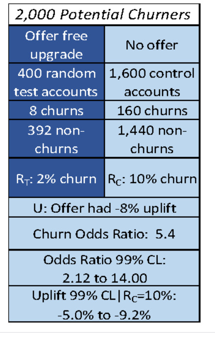
In this experiment, we record 8 churns in the group that received an offer, and 160 churns in the group that did not receive an offer.  This means that there is a 2% churn in the experimental group (RT) and a 10% churn in the control group (RC). The offer has a -8% uplift (U):

Overall Uplift U = RT – RC = 2% – 10% = -8%

The uplift in this case is negative because we are trying to avoid the target behavior rather than promote it.

 For Uplift to be actionable in practice, we also need to know the treatment effect for each individual person uniquely, in addition to the general population.  For example, my previous volume of online shopping may indicate that I am more persuadable to click on a particular advertisement than others in my same demographic group.  Thus, we want to model how the attributes of a case impact the treatment uplift of that case.  The way such a model is created in practice is as follows:

1) predict the outcome with the treatment applied (RTi in the telecom example),

2) predict the outcome without the treatment applied (RCi in the telecom example),

3) calculate the difference in the rates as the uplift (Ui=RTi-RCi), and

4) compute the upper and lower 95% confidence limits on Ui.

Once these values are calculated, individuals can be allocated to the four quadrants of the treatment effect matrix using these rules:

§ If the confidence limits of the Incremental Uplift (Ui) includes zero, the treatment effect can be thought of as unknown and not significant. Regardless of treatment, the Sure Things have a high outcome likelihood and the Lost Causes have a low outcome likelihood.

§ If the Incremental Uplift (Ui) is significantly greater than zero, the predicted outcome increases because of the treatment. These are the Persuadables if the outcome is positive.

§ When the Incremental Uplift (Ui) is significantly less than zero, the predicted outcome is less likely because of the treatment. Traditionally, these are called the Do-Not-Disturbs.

Reference: Mike Thurber. Uplift Modeling: Making Predictive Models Actionable.

[rfmdataanalysis]

Uplift Model

Incremental response models that use a pair of training data sets (treatment and control) measure the incremental effectiveness of direct marketing. These models look for customers who are likely to buy or respond positively to marketing campaigns when they are targeted but are not likely to buy if they are not targeted. The revenue generated from those customers is called incremental revenue.

 The incremental response model divides customers into four groups: (1) those who respond only when targeted with a marketing action, (2) those who respond regardless of contact, (3) those who do not respond, regardless of contact, and (4) those who are less likely to respond because of contact.

 An incremental response model uses two randomly selected data sets, which are called control and treatment as in a clinical trial setting. The treatment group receives the promotion offer, but the control group does not.

In Display 1, the treatment group has a 62% response rate, and the control group has a 33% response rate. The promotion has resulted in about 28% incremental responses and average incremental sales of approximately $26.00. The 28% of customers are called the true responders of the promotion, but you don’t know who they are. Finding those customers is the main purpose of incremental response modeling.

VARIABLE PRESCREENING

Variable selection is an important step in predictive modeling because it reduces the dimension of the model, avoids overfitting, and improves model stability and accuracy. In the context of incremental response modeling, the target is the incremental effect that is calculated as the difference between treatment and control outcomes.

 INCREMENTAL RESPONSE SCORE MODELING

In incremental response modeling, one of the basic models is the difference score model, which measures the differences between predicted values from the model of the treatment group and from the model of the control group. These difference values are called difference scores. The ranked difference scores are binned in descending order for model assessment, and the final top subset is selected as the true responders to the marketing promotion. The predictive model can be built in two different ways: one consists of two separate models from the treatment group and control group, and the other uses a single, combined equation.

 Suppose there are two data sets, and , which are the treatment group and the control group, respectively. Denote a dependent variable and explanatory variables , and denote the number of observations in each group, and . Then,

Without loss of generality, a linear model is considered as follows:

Two models are built separately on

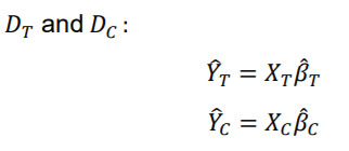
Then, both models are used to calculate predicted values from the entire data sets.

 The difference scores can be obtained from the predicted values as

Customers who have a positive value of are initially considered as the incremental responders as a result of the promotion campaign. However, to determine the final set of incremental responders, further analyses must be performed with the ranked difference scores in decreasing order:

We could build model uses logistic regression with variable selection separately for each model so that each model has more flexibility in regard to its own data set (treatment data and control data).

 INCREMENTAL SALES MODEL

An incremental response model often handles two targets: a binary response and an interval variable such as sales, revenue, and so on. The incremental response model that handles both targets is also known as an incremental sales model. The goal of the incremental sales model is to find customers who are likely to spend incrementally when they receive a promotion.

After two predicted outcome (interval target) models are built from the treatment and control group data sets, the incremental sales model follows the same process as the incremental response model does with the difference scores in order to identify the customers who are likely to spend incrementally when they are targeted by the marketing campaign.

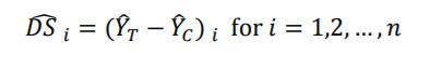
MODEL DIAGNOSTICS

 Model diagnostics can be obtained through a heuristic method by ranking the control and treatment data sets in descending order by the difference score ( ̂ ). The ranked observations are divided into bins. If the number of bins is 10, the bins are deciles. For each bin, the average predicted values are calculated from both the treatment model and the control model. The predicted incremental response is the difference between the two average predicted values for each bin. Similarly, for each bin, the average observed responses are calculated from both models and the observed incremental response accordingly. Display 2 shows the model diagnostics from the estimated response model, which uses the example data set without prescreening variables.

To constitute a good incremental response model, the top percentiles of actual data should have higher incremental rates, and the bottom percentiles should have lower incremental rates. In addition, the rates should decrease monotonically from the top to the bottom percentiles. According to this criterion, the table in Display 2 shows that the estimated model is reasonably good, as expected from the data generation. No percentiles violate the monotonicity. The prediction power of the model is also good enough, which means that the differences between the estimated and actual incremental response rates are small at all the percentiles. The same diagnostic method can be applied for the incremental sales model. The data are sorted in decreasing order by the predicted incremental sales (difference scores in sales prediction), and the ranked observations are binned by using the predefined number of bins. Average values for each bin are calculated from both predicted and observed values. The binned incremental sales should decrease monotonically in a well-fitted incremental model.

In this example, the observed increment does not decrease monotonically; the values between the 30th and 50th percentiles are in increasing order. So this model is not good enough. A better model might be considered by tweaking some of model parameters. However, the model is not too bad, because the incremental values at the top 10th and 20th percentiles are higher than those at the bottom percentiles. The predicted values at all bins slightly miss the actual values. In summary, for the model diagnostics, use the observed incremental value; then (1) compare top percentiles with bottom percentiles, (2) check the decreasing monotonicity, and (3) observe how close the predicted value is to the actual value.

 INCREMENTAL REVENUE AND PROFIT ANALYSIS

Constant Revenue and Constant Cost Consider a simple direct marketing campaign for one product. Assume that the response is the product purchase, the quantity is only one per customer, the marketing cost is $2.00, the product cost is $10.00, and the product price that the customer pays is $40.00. Under these assumptions, you want to decide which customers are in the most profitable group in terms of incremental response. Hereafter, the terms of revenue and profit are exchangeable because they depend on how the cost (expense) is defined. The property setting in Display 4 sets up the analysis.

The Sales and Cost variables shouldn’t be used in the variable setting. As Display 5 shows, you can get profitable customers up to the top 40 percentiles by using the estimated incremental response model. The average profit is also shown for each percentile.

References: Incremental Response Modeling Using SAS® Enterprise Miner™ Taiyeong Lee, Ruiwen Zhang, Xiangxiang Meng, and Laura Ryan SAS Institute Inc.

[rfmdataanalysis]

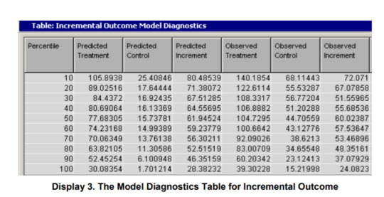
Confusion Matrix & AUC-ROC

Probability of Predictions

A machine learning classification model can be used to predict the actual class of the data point directly or predict its probability of belonging to different classes. The latter gives us more control over the result. We can determine our own threshold to interpret the result of the classifier. This is sometimes more prudent than just building a completely new model!

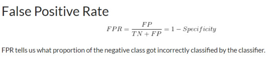
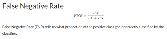
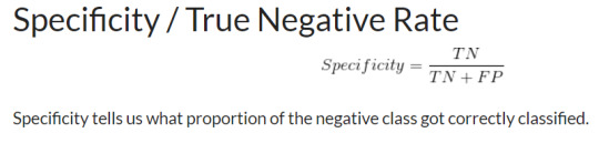
Setting different thresholds for classifying positive class for data points will inadvertently change the Sensitivity and Specificity of the model. And one of these thresholds will probably give a better result than the others, depending on whether we are aiming to lower the number of False Negatives or False Positives.

Have a look at the table below:

The metrics change with the changing threshold values. We can generate different confusion matrices and compare the various metrics that we discussed in the previous section. But that would not be a prudent thing to do. Instead, what we can do is generate a plot between some of these metrics so that we can easily visualize which threshold is giving us a better result.

The AUC-ROC curve solves just that problem!

The Receiver Operator Characteristic (ROC) curve is an evaluation metric for binary classification problems. It is a probability curve that plots the TPR against FPR at various threshold values and essentially separates the ‘signal’ from the ‘noise’. The Area Under the Curve (AUC) is the measure of the ability of a classifier to distinguish between classes and is used as a summary of the ROC curve.

The higher the AUC, the better the performance of the model at distinguishing between the positive and negative classes.

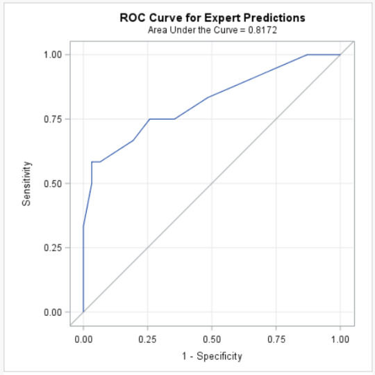
When 0.5<AUC<1, there is a high chance that the classifier will be able to distinguish the positive class values from the negative class values.

When AUC=0.5, then the classifier is not able to distinguish between Positive and Negative class points. Meaning either the classifier is predicting random class or constant class for all the data points.

Reference:

Aniruddha Bhandari.  AUC-ROC Curve in Machine Learning Clearly Explained.