sbrocks99

[sbrocks99]

Running a k-means Cluster Analysis

A k-means cluster analysis was conducted to identify underlying subgroups of adolescents based on their similarity of responses on 11 variables that represent characteristics that could have an impact on school achievement. 

Clustering variables included two binary variables measuring whether or not the adolescent had ever used alcohol or marijuana, as well as quantitative variables measuring alcohol problems, a scale measuring engaging in deviant behaviors (such as vandalism, other property damage, lying, stealing, running away, driving without permission, selling drugs, and skipping school), and scales measuring violence, depression, self-esteem, parental presence, parental activities, family connectedness, and school connectedness. All clustering variables were standardized to have a mean of 0 and a standard deviation of 1.

Data were randomly split into a training set that included 70% of the observations (N=3201) and a test set that included 30% of the observations (N=1701). A series of k-means cluster analyses were conducted on the training data specifying k=1-9 clusters, using Euclidean distance. The variance in the clustering variables that was accounted for by the clusters (r-square) was plotted for each of the nine cluster solutions in an elbow curve to provide guidance for choosing the number of clusters to interpret.

Figure 1. Elbow curve of r-square values for the nine cluster solutions

The elbow curve was inconclusive, suggesting that the 2, 4 and 8-cluster solutions might be interpreted. The results below are for an interpretation of the 4-cluster solution.

Canonical discriminant analyses was used to reduce the 11 clustering variable down a few variables that accounted for most of the variance in the clustering variables. A scatterplot of the first two canonical variables by cluster (Figure 2 shown below) indicated that the observations in clusters 1 and 4 were densely packed with relatively low within cluster variance, and did not overlap very much with the other clusters. 

Cluster 2 was generally distinct, but the observations had greater spread suggesting higher within cluster variance. Observations in cluster 3 were spread out more than the other clusters, showing high within cluster variance. The results of this plot suggest that the best cluster solution may have fewer than 4 clusters, so it will be especially important to also evaluate the cluster solutions with fewer than 4 clusters.

Figure 2. Plot of the first two canonical variables for the clustering variables by cluster.

The means on the clustering variables showed that, compared to the other clusters, adolescents in cluster 1 had moderate levels on the clustering variables. They had a relatively low likelihood of using alcohol or marijuana, but moderate levels of depression and self-esteem. They also appeared to have fairly low levels of school connectedness parental presence, parental involvement in activities and family connectedness. With the exception of having a high likelihood of having used alcohol or marijuana, cluster 2 had higher levels on the clustering variables compared to cluster 1, but moderate compared to clusters 3 and 4. 

On the other hand, cluster 3 clearly included the most troubled adolescents. Adolescents in cluster three had the highest likelihood of having used alcohol, a very high likelihood of having used marijuana, more alcohol problems, and more engagement in deviant and violent behaviors compared to the other clusters. They also had higher levels of depression, lower self-esteem, and the lowest levels of school connectedness, parental presence, involvement of parents in activities, and family connectedness. 

Cluster 4 appeared to include the least troubled adolescents. Compared to adolescents in the other clusters, they were least likely to have used alcohol and marijuana, and had the lowest number of alcohol problems, and deviant and violent behavior. They also had the lowest levels of depression, and higher self-esteem, school connectedness, parental presence, parental involvement in activities and family connectedness.

In order to externally validate the clusters, an Analysis of Variance (ANOVA) was conducting to test for significant differences between the clusters on grade point average (GPA). A tukey test was used for post hoc comparisons between the clusters. Results indicated significant differences between the clusters on GPA (F(3, 3197)=82.28, p<.0001). The tukey post hoc comparisons showed significant differences between clusters on GPA, with the exception that clusters 1 and 2 were not significantly different from each other. Adolescents in cluster 4 had the highest GPA (mean=2.99, sd=0.71), and cluster 3 had the lowest GPA (mean=2.36, sd=0.78).

Complete Code

from pandas import Series, DataFrame import pandas as pd import numpy as np import matplotlib.pylab as plt from sklearn.cross_validation import train_test_split from sklearn import preprocessing from sklearn.cluster import KMeans

""" Data Management """ data = pd.read_csv("tree_addhealth.csv")

#upper-case all DataFrame column names data.columns = map(str.upper, data.columns)

# Data Management

data_clean = data.dropna()

# subset clustering variables cluster=data_clean[['ALCEVR1','MAREVER1','ALCPROBS1','DEVIANT1','VIOL1', 'DEP1','ESTEEM1','SCHCONN1','PARACTV', 'PARPRES','FAMCONCT']] cluster.describe()

# standardize clustering variables to have mean=0 and sd=1 clustervar=cluster.copy() clustervar['ALCEVR1']=preprocessing.scale(clustervar['ALCEVR1'].astype('float64')) clustervar['ALCPROBS1']=preprocessing.scale(clustervar['ALCPROBS1'].astype('float64')) clustervar['MAREVER1']=preprocessing.scale(clustervar['MAREVER1'].astype('float64')) clustervar['DEP1']=preprocessing.scale(clustervar['DEP1'].astype('float64')) clustervar['ESTEEM1']=preprocessing.scale(clustervar['ESTEEM1'].astype('float64')) clustervar['VIOL1']=preprocessing.scale(clustervar['VIOL1'].astype('float64')) clustervar['DEVIANT1']=preprocessing.scale(clustervar['DEVIANT1'].astype('float64')) clustervar['FAMCONCT']=preprocessing.scale(clustervar['FAMCONCT'].astype('float64')) clustervar['SCHCONN1']=preprocessing.scale(clustervar['SCHCONN1'].astype('float64')) clustervar['PARACTV']=preprocessing.scale(clustervar['PARACTV'].astype('float64')) clustervar['PARPRES']=preprocessing.scale(clustervar['PARPRES'].astype('float64'))

# split data into train and test sets clus_train, clus_test = train_test_split(clustervar, test_size=.3, random_state=123)

# k-means cluster analysis for 1-9 clusters                                                           from scipy.spatial.distance import cdist clusters=range(1,10) meandist=[]

for k in clusters:    model=KMeans(n_clusters=k)    model.fit(clus_train)    clusassign=model.predict(clus_train)    meandist.append(sum(np.min(cdist(clus_train, model.cluster_centers_, 'euclidean'), axis=1))    / clus_train.shape[0])

""" Plot average distance from observations from the cluster centroid to use the Elbow Method to identify number of clusters to choose """

plt.plot(clusters, meandist) plt.xlabel('Number of clusters') plt.ylabel('Average distance') plt.title('Selecting k with the Elbow Method')

# Interpret 3 cluster solution model3=KMeans(n_clusters=3) model3.fit(clus_train) clusassign=model3.predict(clus_train) # plot clusters

from sklearn.decomposition import PCA pca_2 = PCA(2) plot_columns = pca_2.fit_transform(clus_train) plt.scatter(x=plot_columns[:,0], y=plot_columns[:,1], c=model3.labels_,) plt.xlabel('Canonical variable 1') plt.ylabel('Canonical variable 2') plt.title('Scatterplot of Canonical Variables for 3 Clusters') plt.show()

""" BEGIN multiple steps to merge cluster assignment with clustering variables to examine cluster variable means by cluster """ # create a unique identifier variable from the index for the # cluster training data to merge with the cluster assignment variable clus_train.reset_index(level=0, inplace=True) # create a list that has the new index variable cluslist=list(clus_train['index']) # create a list of cluster assignments labels=list(model3.labels_) # combine index variable list with cluster assignment list into a dictionary newlist=dict(zip(cluslist, labels)) newlist # convert newlist dictionary to a dataframe newclus=DataFrame.from_dict(newlist, orient='index') newclus # rename the cluster assignment column newclus.columns = ['cluster']

# now do the same for the cluster assignment variable # create a unique identifier variable from the index for the # cluster assignment dataframe # to merge with cluster training data newclus.reset_index(level=0, inplace=True) # merge the cluster assignment dataframe with the cluster training variable dataframe # by the index variable merged_train=pd.merge(clus_train, newclus, on='index') merged_train.head(n=100) # cluster frequencies merged_train.cluster.value_counts()

""" END multiple steps to merge cluster assignment with clustering variables to examine cluster variable means by cluster """

# FINALLY calculate clustering variable means by cluster clustergrp = merged_train.groupby('cluster').mean() print ("Clustering variable means by cluster") print(clustergrp)

# validate clusters in training data by examining cluster differences in GPA using ANOVA # first have to merge GPA with clustering variables and cluster assignment data gpa_data=data_clean['GPA1'] # split GPA data into train and test sets gpa_train, gpa_test = train_test_split(gpa_data, test_size=.3, random_state=123) gpa_train1=pd.DataFrame(gpa_train) gpa_train1.reset_index(level=0, inplace=True) merged_train_all=pd.merge(gpa_train1, merged_train, on='index') sub1 = merged_train_all[['GPA1', 'cluster']].dropna()

import statsmodels.formula.api as smf import statsmodels.stats.multicomp as multi

gpamod = smf.ols(formula='GPA1 ~ C(cluster)', data=sub1).fit() print (gpamod.summary())

print ('means for GPA by cluster') m1= sub1.groupby('cluster').mean() print (m1)

print ('standard deviations for GPA by cluster') m2= sub1.groupby('cluster').std() print (m2)

mc1 = multi.MultiComparison(sub1['GPA1'], sub1['cluster']) res1 = mc1.tukeyhsd() print(res1.summary())

[sbrocks99]

Running a Lasso Regression Analysis

Hey guy’s so far we have seen how to run classification trees and random forest analysis. So now let's see how we test a Lasso regression model in Python.

First, I will call in the libraries that I will need. In addition to the pandas, numpy, and matplotlib libraries I'll need the train_test_split function from the sklearn.cross_validation library, and the LassoLarsCV function from the sklearn.linear_model library. 

After I call in the data set using the pd.read_csv function, I'll do a little extra data management. Namely, I want to create a new dataset called data_clean in which I will delete observations with missing data on any of the variables using the dropna function.

Then, I want to create a variable for gender called male, that is coded zero for female and one for male, like the other binary variables in the data set.

#from pandas import Series, DataFrame import pandas as pd import numpy as np import matplotlib.pylab as plt from sklearn.cross_validation import train_test_split from sklearn.linear_model import LassoLarsCV

#Load the dataset data = pd.read_csv("tree_addhealth.csv")

#upper-case all DataFrame column names data.columns = map(str.upper, data.columns)

# Data Management data_clean = data.dropna() recode1 = {1:1, 2:0} data_clean['MALE']= data_clean['BIO_SEX'].map(recode1)

Next, I will create two data frames. The first, called predvar, P-R-E-D-V-A-R, will include only the predictor variables that I will use in the lasso regression model. The second, called target, will include only my school connectedness response variable.

#select predictor variables and target variable as separate data sets   predvar= data_clean[['MALE','HISPANIC','WHITE','BLACK','NAMERICAN','ASIAN', 'AGE','ALCEVR1','ALCPROBS1','MAREVER1','COCEVER1','INHEVER1','CIGAVAIL','DEP1', 'ESTEEM1','VIOL1','PASSIST','DEVIANT1','GPA1','EXPEL1','FAMCONCT','PARACTV', 'PARPRES']]

target = data_clean.SCHCONN1

In lasso regression, the penalty term is not fair if the predictive variables are not on the same scale, meaning that not all the predictors get the same penalty. So I will standardize all the predictors to have a mean equal to zero and a standard deviation equal to one, including my binary predictors, which will put them all on the same scale. 

To standardize the predictors, I'm going to first create a copy of my predvar data frame and name it predictors. Then, I'm going to import the preprocessing function from the sklearn library. 

# standardize predictors to have mean=0 and sd=1 predictors=predvar.copy()

I will list the name of my predictor variable = preprocessing.scale. The preprocessing.scale function transforms the variable to have a mean of zero and a standard deviation of one, thus putting all the predictors on the same scale. Then, in parentheses I type the name of my variable again, and add .astype('float64'). The as type float 64 code ensures that my predictors will have a numeric format.

from sklearn import preprocessing predictors['MALE']=preprocessing.scale(predictors['MALE'].astype('float64')) predictors['HISPANIC']=preprocessing.scale(predictors['HISPANIC'].astype('float64')) predictors['WHITE']=preprocessing.scale(predictors['WHITE'].astype('float64')) predictors['NAMERICAN']=preprocessing.scale(predictors['NAMERICAN'].astype('float64')) predictors['ASIAN']=preprocessing.scale(predictors['ASIAN'].astype('float64')) predictors['AGE']=preprocessing.scale(predictors['AGE'].astype('float64')) predictors['ALCEVR1']=preprocessing.scale(predictors['ALCEVR1'].astype('float64')) predictors['ALCPROBS1']=preprocessing.scale(predictors['ALCPROBS1'].astype('float64')) predictors['MAREVER1']=preprocessing.scale(predictors['MAREVER1'].astype('float64')) predictors['COCEVER1']=preprocessing.scale(predictors['COCEVER1'].astype('float64')) predictors['INHEVER1']=preprocessing.scale(predictors['INHEVER1'].astype('float64')) predictors['CIGAVAIL']=preprocessing.scale(predictors['CIGAVAIL'].astype('float64')) predictors['DEP1']=preprocessing.scale(predictors['DEP1'].astype('float64')) predictors['ESTEEM1']=preprocessing.scale(predictors['ESTEEM1'].astype('float64')) predictors['VIOL1']=preprocessing.scale(predictors['VIOL1'].astype('float64')) predictors['PASSIST']=preprocessing.scale(predictors['PASSIST'].astype('float64')) predictors['DEVIANT1']=preprocessing.scale(predictors['DEVIANT1'].astype('float64')) predictors['GPA1']=preprocessing.scale(predictors['GPA1'].astype('float64')) predictors['EXPEL1']=preprocessing.scale(predictors['EXPEL1'].astype('float64')) predictors['FAMCONCT']=preprocessing.scale(predictors['FAMCONCT'].astype('float64')) predictors['PARACTV']=preprocessing.scale(predictors['PARACTV'].astype('float64')) predictors['PARPRES']=preprocessing.scale(predictors['PARPRES'].astype('float64'))

In the next line of code, I will use the train test split function from the sklearn cross validation library to randomly split my data set into a training data set consisting of 70% of the total observations in the data set. And a test data set consisting of the other 30% of the observations. First, I list the two training data sets. 

The first data set, called pred_train, will include the predictor variables from my training data set and a second data set, called pred_test, will include the predictor variables from my test data set. The third data set, called tar_train, will include the response variable from my training data set and the fourth data set, called tar_test, will include the response variable for my test data set. 

Then I type the function name, train_test_split and in parentheses, I list my full predictors and target data set names with commas separating them. The test_size option tells Python to randomly place 30% of the observations in the pred_test and pred_tar test data sets. By default, the other 70% of the observations are placed in the pred_train and tar_train training data sets. 

The random_state option specifies a random number seed to ensure that the data are randomly split the same way if I run the code again.

# split data into train and test sets pred_train, pred_test, tar_train, tar_test = train_test_split(predictors, target, test_size=.3, random_state=123)

Complete Code

#from pandas import Series, DataFrame import pandas as pd import numpy as np import matplotlib.pylab as plt from sklearn.cross_validation import train_test_split from sklearn.linear_model import LassoLarsCV

#Load the dataset data = pd.read_csv("tree_addhealth.csv")

#upper-case all DataFrame column names data.columns = map(str.upper, data.columns)

# Data Management data_clean = data.dropna() recode1 = {1:1, 2:0} data_clean['MALE']= data_clean['BIO_SEX'].map(recode1)

#select predictor variables and target variable as separate data sets   predvar= data_clean[['MALE','HISPANIC','WHITE','BLACK','NAMERICAN','ASIAN', 'AGE','ALCEVR1','ALCPROBS1','MAREVER1','COCEVER1','INHEVER1','CIGAVAIL','DEP1', 'ESTEEM1','VIOL1','PASSIST','DEVIANT1','GPA1','EXPEL1','FAMCONCT','PARACTV', 'PARPRES']]

target = data_clean.SCHCONN1

# standardize predictors to have mean=0 and sd=1 predictors=predvar.copy() from sklearn import preprocessing predictors['MALE']=preprocessing.scale(predictors['MALE'].astype('float64')) predictors['HISPANIC']=preprocessing.scale(predictors['HISPANIC'].astype('float64')) predictors['WHITE']=preprocessing.scale(predictors['WHITE'].astype('float64')) predictors['NAMERICAN']=preprocessing.scale(predictors['NAMERICAN'].astype('float64')) predictors['ASIAN']=preprocessing.scale(predictors['ASIAN'].astype('float64')) predictors['AGE']=preprocessing.scale(predictors['AGE'].astype('float64')) predictors['ALCEVR1']=preprocessing.scale(predictors['ALCEVR1'].astype('float64')) predictors['ALCPROBS1']=preprocessing.scale(predictors['ALCPROBS1'].astype('float64')) predictors['MAREVER1']=preprocessing.scale(predictors['MAREVER1'].astype('float64')) predictors['COCEVER1']=preprocessing.scale(predictors['COCEVER1'].astype('float64')) predictors['INHEVER1']=preprocessing.scale(predictors['INHEVER1'].astype('float64')) predictors['CIGAVAIL']=preprocessing.scale(predictors['CIGAVAIL'].astype('float64')) predictors['DEP1']=preprocessing.scale(predictors['DEP1'].astype('float64')) predictors['ESTEEM1']=preprocessing.scale(predictors['ESTEEM1'].astype('float64')) predictors['VIOL1']=preprocessing.scale(predictors['VIOL1'].astype('float64')) predictors['PASSIST']=preprocessing.scale(predictors['PASSIST'].astype('float64')) predictors['DEVIANT1']=preprocessing.scale(predictors['DEVIANT1'].astype('float64')) predictors['GPA1']=preprocessing.scale(predictors['GPA1'].astype('float64')) predictors['EXPEL1']=preprocessing.scale(predictors['EXPEL1'].astype('float64')) predictors['FAMCONCT']=preprocessing.scale(predictors['FAMCONCT'].astype('float64')) predictors['PARACTV']=preprocessing.scale(predictors['PARACTV'].astype('float64')) predictors['PARPRES']=preprocessing.scale(predictors['PARPRES'].astype('float64'))

# split data into train and test sets pred_train, pred_test, tar_train, tar_test = train_test_split(predictors, target,                                                              test_size=.3, random_state=123)

# specify the lasso regression model model=LassoLarsCV(cv=10, precompute=False).fit(pred_train,tar_train)

# print variable names and regression coefficients dict(zip(predictors.columns, model.coef_))

# plot coefficient progression m_log_alphas = -np.log10(model.alphas_) ax = plt.gca() plt.plot(m_log_alphas, model.coef_path_.T) plt.axvline(-np.log10(model.alpha_), linestyle='--', color='k',            label='alpha CV') plt.ylabel('Regression Coefficients') plt.xlabel('-log(alpha)') plt.title('Regression Coefficients Progression for Lasso Paths')

# plot mean square error for each fold m_log_alphascv = -np.log10(model.cv_alphas_) plt.figure() plt.plot(m_log_alphascv, model.cv_mse_path_, ':') plt.plot(m_log_alphascv, model.cv_mse_path_.mean(axis=-1), 'k',         label='Average across the folds', linewidth=2) plt.axvline(-np.log10(model.alpha_), linestyle='--', color='k',            label='alpha CV') plt.legend() plt.xlabel('-log(alpha)') plt.ylabel('Mean squared error') plt.title('Mean squared error on each fold')

# MSE from training and test data from sklearn.metrics import mean_squared_error train_error = mean_squared_error(tar_train, model.predict(pred_train)) test_error = mean_squared_error(tar_test, model.predict(pred_test)) print ('training data MSE') print(train_error) print ('test data MSE') print(test_error)

# R-square from training and test data rsquared_train=model.score(pred_train,tar_train) rsquared_test=model.score(pred_test,tar_test) print ('training data R-square') print(rsquared_train) print ('test data R-square') print(rsquared_test)

[sbrocks99]

Running a Random Forest

Hey guy’s welcome back in previous blog we have seen that, how to run classification trees in python you can check it here. In this blog you are going to learn how to run Random Forest using python.

So now let's see how to generate a random forest with Python. Again, I'm going to use the Wave One, Add Health Survey that I have data managed for the purpose of growing decision trees. You'll recall that there are several variables. Again, we'll define the response or target variable, regular smoking, based on answers to the question, have you ever smoked cigarettes regularly? That is, at least one cigarette every day for 30 days. 

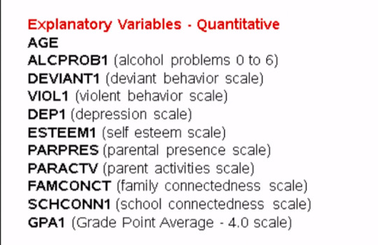
The candidate explanatory variables include gender, race, alcohol, marijuana, cocaine, or inhalant use. Availability of cigarettes in the home, whether or not either parent was on public assistance, any experience with being expelled from school, age, alcohol problems, deviance, violence, depression, self esteem, parental presence, activities with parents family and school connectedness and grade point average. 

Much of the code that we'll write for our random forest will be quite similar to the code we had written for individual decision trees.

First there are a number of libraries that we need to call in, including features from the sklearn library.

from pandas import Series, DataFrame import pandas as pd import numpy as np import os import matplotlib.pylab as plt from sklearn.cross_validation import train_test_split from sklearn.tree import DecisionTreeClassifier from sklearn.metrics import classification_report import sklearn.metrics # Feature Importance from sklearn import datasets from sklearn.ensemble import ExtraTreesClassifier

Next I'm going to use the change working directory function from the OS library to indicate where my data set is located.

os.chdir("C:\TREES")

Next I'll load my data set called tree_addhealth.csv. because decision tree analyses cannot handle any NAs in our data set, my next step is to create a clean data frame that drops all NAs. Setting the new data frame called data_clean I can now take a look at various characteristics of my data, by using the D types and describe functions to examine data types and summary statistics.

#Load the dataset

AH_data = pd.read_csv("tree_addhealth.csv") data_clean = AH_data.dropna()

data_clean.dtypes data_clean.describe()

Next I set my explanatory and response, or target variables, and then include the train test split function for predictors and target. And set the size ratio to 60% for the training sample, and 40% for the test sample by indicating test_size=.4.

#Split into training and testing sets

predictors = data_clean[['BIO_SEX','HISPANIC','WHITE','BLACK','NAMERICAN','ASIAN','age', 'ALCEVR1','ALCPROBS1','marever1','cocever1','inhever1','cigavail','DEP1','ESTEEM1','VIOL1', 'PASSIST','DEVIANT1','SCHCONN1','GPA1','EXPEL1','FAMCONCT','PARACTV','PARPRES']]

targets = data_clean.TREG1

Here I request the shape of these predictor and target and training test samples.

pred_train.shape pred_test.shape tar_train.shape tar_test.shape

From sklearn.ensamble I import the RandomForestClassifier

#Build model on training data from sklearn.ensemble import RandomForestClassifier

Now that training and test data sets have already been created, we'll initialize the random forest classifier from SK Learn and indicate n_estimators=25. n_estimators are the number of trees you would build with the random forest algorithm.

classifier=RandomForestClassifier(n_estimators=25)

Next I actually fit the model with the classifier.fit function which we passed the training predictors and training targets too.

classifier=classifier.fit(pred_train,tar_train)

Then, we go unto the prediction on the testator set. And we could also similar to decision tree code as for the confusion matrix and accuracy scores.

predictions=classifier.predict(pred_test)

sklearn.metrics.confusion_matrix(tar_test,predictions) sklearn.metrics.accuracy_score(tar_test, predictions)

For the confusion matrix, we see the true negatives and true positives on the diagonal. And the 207 and the 82 represent the false negatives and false positives, respectively. Notice that the overall accuracy for the forest is 0.84. So 84% of the individuals were classified correctly, as regular smokers, or not regular smokers.

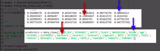
Given that we don't interpret individual trees in a random forest, the most helpful information to be gotten from a forest is arguably the measured importance for each explanatory variable. Also called the features. Based on how many votes or splits each has produced in the 25 tree ensemble. To generate importance scores, we initialize the extra tree classifier, and then fit a model. Finally, we ask Python to print the feature importance scores calculated from the forest of trees that we've grown.

# fit an Extra Trees model to the data model = ExtraTreesClassifier() model.fit(pred_train,tar_train) # display the relative importance of each attribute print(model.feature_importances_)

The variables are listed in the order they've been named earlier in the code. Starting with gender, called BIO_SEX, and ending with parental presence. As we can see the variables with the highest important score at 0.13 is marijuana use. And the variable with the lowest important score is Asian ethnicity at .006.

As you will recall, the correct classification rate for the random forest was 84%. So were 25 trees actually needed to get this correct rate of classification? To determine what growing larger number of trees has brought us in terms of correct classification. We're going to use code that builds for us different numbers of trees, from one to 25, and provides the correct classification rate for each. This code will build for us random forest classifier from one to 25, and then finding the accuracy score for each of those trees from one to 25, and storing it in an array. This will give me 25 different accuracy values. And we'll plot them as the number of trees increase.

""" Running a different number of trees and see the effect of that on the accuracy of the prediction """

trees=range(25) accuracy=np.zeros(25)

for idx in range(len(trees)):   classifier=RandomForestClassifier(n_estimators=idx + 1)   classifier=classifier.fit(pred_train,tar_train)   predictions=classifier.predict(pred_test)   accuracy[idx]=sklearn.metrics.accuracy_score(tar_test, predictions)

plt.cla() plt.plot(trees, accuracy)

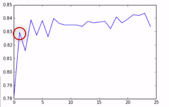
As you can see, with only one tree the accuracy is about 83%, and it climbs to only about 84% with successive trees that are grown giving us some confidence that it may be perfectly appropriate to interpret a single decision tree for this data. Given that it's accuracy is quite near that of successive trees in the forest. 

To summarize, like decision trees, random forests are a type of data mining algorithm that can select from among a large number of variables. Those that are most important in determining the target or response variable to be explained.

Also light decision trees. The target variable in a random forest can be categorical or quantitative. And the group of explanatory variables or features can be categorical and quantitative in any combination. Unlike decision trees however, the results of random forests often generalize well to new data. 

Since the strongest signals are able to emerge through the growing of many trees. Further, small changes in the data do not impact the results of a random forest. In my opinion, the main weakness of random forests is simply that the results are less satisfying, since no trees are actually interpreted. Instead, the forest of trees is used to rank the importance of variables in predicting the target.

Thus we get a sense of the most important predictive variables but not necessarily their relationships to one another.

Complete Code

from pandas import Series, DataFrame import pandas as pd import numpy as np import os import matplotlib.pylab as plt from sklearn.cross_validation import train_test_split from sklearn.tree import DecisionTreeClassifier from sklearn.metrics import classification_report import sklearn.metrics # Feature Importance from sklearn import datasets from sklearn.ensemble import ExtraTreesClassifier

os.chdir("C:\TREES")

#Load the dataset

AH_data = pd.read_csv("tree_addhealth.csv") data_clean = AH_data.dropna()

data_clean.dtypes data_clean.describe()

#Split into training and testing sets

predictors = data_clean[['BIO_SEX','HISPANIC','WHITE','BLACK','NAMERICAN','ASIAN','age', 'ALCEVR1','ALCPROBS1','marever1','cocever1','inhever1','cigavail','DEP1','ESTEEM1','VIOL1', 'PASSIST','DEVIANT1','SCHCONN1','GPA1','EXPEL1','FAMCONCT','PARACTV','PARPRES']]

targets = data_clean.TREG1

pred_train, pred_test, tar_train, tar_test  = train_test_split(predictors, targets, test_size=.4)

pred_train.shape pred_test.shape tar_train.shape tar_test.shape

#Build model on training data from sklearn.ensemble import RandomForestClassifier

classifier=RandomForestClassifier(n_estimators=25) classifier=classifier.fit(pred_train,tar_train)

predictions=classifier.predict(pred_test)

sklearn.metrics.confusion_matrix(tar_test,predictions) sklearn.metrics.accuracy_score(tar_test, predictions)

# fit an Extra Trees model to the data model = ExtraTreesClassifier() model.fit(pred_train,tar_train) # display the relative importance of each attribute print(model.feature_importances_)

""" Running a different number of trees and see the effect of that on the accuracy of the prediction """

trees=range(25) accuracy=np.zeros(25)

for idx in range(len(trees)):   classifier=RandomForestClassifier(n_estimators=idx + 1)   classifier=classifier.fit(pred_train,tar_train)   predictions=classifier.predict(pred_test)   accuracy[idx]=sklearn.metrics.accuracy_score(tar_test, predictions)

plt.cla() plt.plot(trees, accuracy)

If you are still here, I appreciate that, and see you guy’s next time. ✌️

[sbrocks99]

Descision Tree

The National Longitudinal Study of Adolescent Health (AddHealth) is a representative school-based survey of adolescents in grades 7-12 in the United States. The Wave 1 survey focuses on factors that may influence adolescents’ health and risk behaviors, including personal traits, families, friendships, romantic relationships, peer groups, schools, neighborhoods, and communities.

So now let's see how to generate a decision tree with Python. Before we even write the program, there are additional installation steps that need to be made. 

When writing our program, in order to be able to import our data and run and visualize decision trees in Python, there are also a number of libraries that we need to call in, including features from the SKLearn library. 

Importing Libraries

from pandas import Series, DataFrame import pandas as pd import numpy as np import os import matplotlib.pylab as plt from sklearn.cross_validation import train_test_split from sklearn.tree import DecisionTreeClassifier from sklearn.metrics import classification_report import sklearn.metrics

Next, I'm going to use the change working directory function from the os library. To indicate where my data set is located. 

os.chdir("C:\TREES")

Then I'll load my data set, called tree_addheath.csv. 

AH_data = pd.read_csv("tree_addhealth.csv")

Because decision tree analyses cannot handle any NA's in our data set, my next step is to create a clean data frame that drops all NA's.

data_clean = AH_data.dropna()

data_clean.dtypes data_clean.describe()

Setting the new data frame called data_clean, I can now take a look at various characteristics of my data by using the d types and describe functions to examine data types and summary statistics. 

Modeling And Prediction

Next, I set my explanatory and response or target variables. And then include the train test split function for predictors and target. 

#Split into training and testing sets

predictors = data_clean[['BIO_SEX','HISPANIC','WHITE','BLACK','NAMERICAN','ASIAN', 'age','ALCEVR1','ALCPROBS1','marever1','cocever1','inhever1','cigavail','DEP1', 'ESTEEM1','VIOL1','PASSIST','DEVIANT1','SCHCONN1','GPA1','EXPEL1','FAMCONCT','PARACTV', 'PARPRES']]

targets = data_clean.TREG1

And set the size ratio to 60% for the training sample and 40% for the test sample by indicating test_size=.4. 

pred_train, pred_test, tar_train, tar_test  =   train_test_split(predictors, targets, test_size=.4)

Here I request the shape of these predictor and target training and test samples.

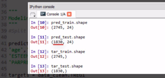
pred_train.shape pred_test.shape tar_train.shape tar_test.shape

The training sample has 2,745 observations or rows, 60% of our original sample, and 24 explanatory variables.

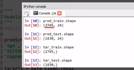
The test sample has 1,830 observations or rows. 40% of the original sample. And again 24 explanatory variables or columns.

Once training and testing data sets have been created, we will initialize the DecisionTreeClassifier from SKLearn. Then use this classifier.fit function which you pass the training predictors and training targets to. It's this code that will fit our model.

#Build model on training data

classifier=DecisionTreeClassifier() classifier=classifier.fit(pred_train,tar_train)

Next we include the predict function where we predict for the test values and then call in the confusion matrix function which we passed the target test sample to.

predictions=classifier.predict(pred_test)

sklearn.metrics.confusion_matrix(tar_test,predictions) sklearn.metrics.accuracy_score(tar_test, predictions)

This shows the correct and incorrect classifications of our decision tree. The diagonal, 1,291 and 117, represent the number of true negative for regular smoking, and the number of true positives, respectively.

The 211, on the bottom left, represents the number of false negatives. Classifying regular smokers as not regular smokers.

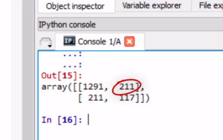
And the 211 on the top right, the number of false positives, classifying a non regular smoker as a regular smoker.

We can also look at the accuracy score which is approximately 0.77, which suggests that the decision tree model has classified 77% of the sample correctly as either regular or not regular smokers.

But what does our decision tree look like? To display the final tree, we need to import more features from the SKLearn and other libraries.

#Displaying the decision tree from sklearn import tree

#from StringIO import StringIO from io import StringIO

#from StringIO import StringIO from IPython.display import Image

out = StringIO() tree.export_graphviz(classifier, out_file=out)

import pydotplus graph=pydotplus.graph_from_dot_data(out.getvalue()) Image(graph.create_png())

Then, with these last three lines of code, we import pi.plus and request the picture of our decision tree.

Conclusion

As we've seen, an advantage of decision trees is they're easy to interpret and visualize especially when the tree is very small. Tree based methods also handle large data-sets well. And can predict both binary, categorical target variables, as shown in our example, and also quantitative target variables. However, as we've also shown, small changes in the data can lead to different splits and this can undermine the interpretability of the model. Also decision trees are not very reproducible on future data.