shadywolfclambiscuit-blog - Tumblr blog

shadywolfclambiscuit-blog · 7 years ago

Text

Writing about the data: Regression Analysis

Hello everyone, after successful completion of two initial module of the course “Data Management and Visualization” and “Data Analysis Tool” now it’s time to continue my Data science learning.

In this blog I will be writing about steps, which I have taken to collect the data, method to collect the data and managing the data for further Regression analysis.

Data collection and data information: To collect the data I searched on google “Raw data for Regression Analysis” and I come across various sources however I found one of the best resource to get the data for all kind of Data science projects Springboard blog. Under this I got the reference of one of the website “Lending Club Statistics” which includes the data for Loan amount transaction and declined loan application.

Method: After reviewing this website and reading the data it seems, data collection process happened in multiple steps:-

· Customer come on web portal and submit the personal loan query and provide basic information

· Representative calls/email back to customer to collect the required document and also asked to provide required details

Customer provides all the personal details along with professional details e.g. location, type of house, salary, about other liability, family and social status etc.

Complete data is being divided into two categories:

1. Data ,for which loan got approved

2. Loan reject data, which does not meet the credit policy

Data, for which loan got approved: This data is being measured across 145 different variables and having 42,535 records out of this 39,786(94%) is for approved loan and remaining 2749(6%) is for those loan which does not meet the credit policy and got rejected. Loan tenure was 3 to 5 years and for different purpose. Geographically this data is from all the states of USA and for all age group people. It contain complete loan data for all loans issued through the time period stated, including the current loan status (Current, Late, Fully Paid, etc.) and latest payment information. Date range for this data is 2007-11 year.

Cleaning and managing the data: Once we explore the data then we can observer there lot of things available into the data which does not make sense to our analysis. To perform the right set of analysis it is required to have correct data. For example assigning the right job categories which will help us to identify that is there issue with any particular job category, also though initially we have observed that there are 145 variables but there are lot of variables which does not have data for further analysis I will be removing them.

Now the next step is to look into the data closely and explore it to the nth level to get the right data to analyze and also identify the confounding variables, exploratory and response variables.

Data can be downloaded for the review from this link: Click Here

Note : Anything which underline that has hyperlink to go to particular web source.

#coursera #python #regressionanalysis

1 note · View note

shadywolfclambiscuit-blog · 7 years ago

Text

Week4: Assignment, Testing a Potential Moderator

o complete this assignment and analysis I would be taking my previous completed analysis.

As we know that while finding association between two variables we have different tests which can be used based on type of selected variable. Just to show my understanding I would be going to run ANOVA which always required while comparing one categorical and one quantetive variable.

I will be running ANOVA test first without considering any potential moderator later on I will be running ANOVA test with the consideration of moderator variable.

Running ANOVA test and its output:

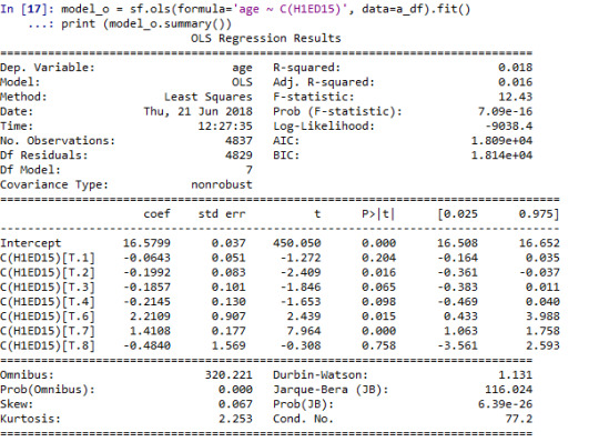
We can observe F-Statistic value 12.43 and p value is .7.09e-16 which is lesser than .05 (p<.05) hence we will reject the null hypothesis and we can say All age people are getting along with teacher have difference in their mean.

Now we will introduce potential moderate variable which is Gender in my analysis.

I will be creating subset of the data based on Gender, dataset is being created for male and female respectively.

Running Analysis for Male:

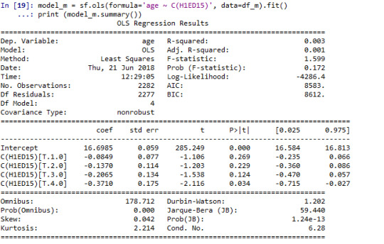
We can observe F-Statistic value 1.59 and p value is .17 which is greater than .05 (p<.05) hence we will fail to reject the null hypothesis and we can say All age Male people are getting along with teacher have almost same mean.

Running Analysis for Female:

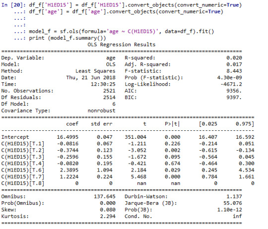
We can observe F-Statistic value 8.44 and p value is 4.30e-09 which is lesser than .05 (p<.05) hence we will reject the null hypothesis and we can say All age female are getting along with teacher have difference in their mean.

Conclusion:

We have performed ANOVA Test in whole dataset and observed that all age people are getting along with teacher have difference in their mean.

However when we introduce the Gender as moderator we can see a change in our analysis and now we can say that Male are getting along with teacher not having difference in their mean but males are having difference.

Similar we can see other test after using moderator and observe is their change or not.

#coursera #python

0 notes

shadywolfclambiscuit-blog · 7 years ago

Text

Week 3: Assignment of Correlations

To complete our analysis we are choosing Gapminder dataset and the variables 'incomeperperson', 'alcconsumption', 'co2emissions' and 'oilperperson'.

To test the association between 2 variables we have an option to choose the test, as we are going to analyze to Quantetive variables then we can narrow down our research and choose correlation test, however we have option to use scatter plot only but that will not give complete information so in addition to that we need find out the correlation coefficient (r) and to get exact variability we have to get the r-square (r2).

Let’ see the association of Income per person with Alcohol consumption, Co2 emissions and oil per person.

Image 1:

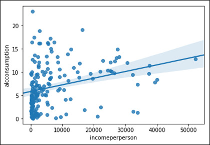
Image 2:

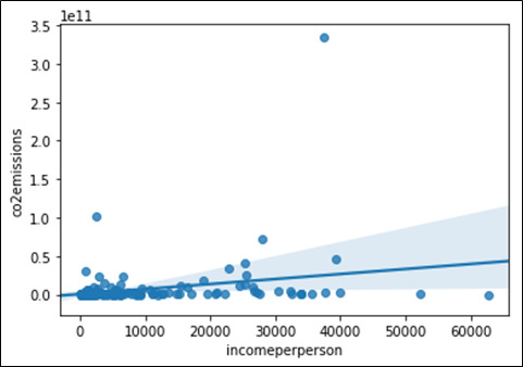
Image 3:

By looking at all the three scatter plot we can say there is correlation between two variables but how strong or weak it is we cannot say, because in image 2 and 3 almost all the values are much closer to the fit line as compare to image 3. To understand how strong association is we have to perform some additional test. Letâ€™s get the p-value and correlation coefficient to prove the association between variables.

Output for Image 1: Association between Income per person and Alcohol consumption

r = 0.13

p = 0.31

Insights: Here we can see our correlation coefficient r is .13 and p value is .31, hence we are fail to reject the null hypothesis and can say there is association between Income per person and Alcohol consumption however correlation coefficient is .13 which shows weak positive correlation.

Output for Image 1: Association between Income per person and Co2 emissions

r = 0.29

p = 0.02

Insights: Here we can see our correlation coefficient r is .29 and p value is .02, hence we will reject the null hypothesis and can say there is no association between Income per person and Co2 emissions however correlation coefficient is .29 which cannot be further utilized as these are statistically correlated.

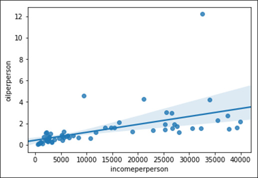
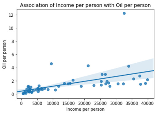
Output for Image 1: Association between Income per person and Oil per person

r = 0.54

p = 0.31

Insights: Here we can see our correlation coefficient r is .54 and p value is .31, hence we will fail to reject the null hypothesis and can say there is association between Income per person and Oil per person however correlation coefficient is .54 which is closer 1 so we can that there is strong positive correlations,

In the nut shall we can say Income per person is directly impacting the Oil per person positively, it mean if ones increased other also start increasing.

****************************Used python Code*************************************

# -*- coding: utf-8 -*- """ Created on Sun Jun 10 11:44:12 2018

@author: Nikhil Tripathi """

import pandas as pd import numpy as ny import seaborn as sn import matplotlib.pyplot as plt import scipy as sy

#Reading gapminder dataset data1 = pd.read_csv('Gapminder.csv,low_memory = False') print(data1.head(10))

#Creating subset with required variable only s_data = data1[['incomeperperson','alcconsumption','co2emissions','oilperperson']]

#Describing the datasets s_data.describe()

#Coverting variable into numeric s_data['incomeperperson'] = s_data['incomeperperson'].convert_objects(convert_numeric = True) s_data['alcconsumption'] = s_data['alcconsumption'].convert_objects(convert_numeric = True) s_data['co2emissions'] = s_data['co2emissions'].convert_objects(convert_numeric = True) s_data['oilperperson'] = s_data['oilperperson'].convert_objects(convert_numeric = True)

s_data['incomeperperson'].describe() s_data['alcconsumption'].describe() s_data['co2emissions'].describe() s_data['oilperperson'].describe()

#Lets Find out the Correlation of Incomeperperson with alcconsuption, co2emissions and oilperperson sctr_plt1 = sn.regplot(x = 'incomeperperson', y = 'alcconsumption', fit_reg = True, data = s_data) sctr_plt2 = sn.regplot(x = 'incomeperperson', y = 'co2emissions', fit_reg = True, data = s_data) sctr_plt3 = sn.regplot(x = 'incomeperperson', y = 'oilperperson', fit_reg = True, data = s_data)

# Removing all the na values from the dataset or selected columns s_data_1 = s_data.dropna()

print ('Association between Income per person and Alcohol consumption') print (sy.stats.pearsonr(s_data_1['incomeperperson'], s_data_1['alcconsumption']))

print ('Association between Income per person and Co2 emissions') print (sy.stats.pearsonr(s_data_1['incomeperperson'], s_data_1['co2emissions']))

print ('Association between Income per person and Oil per person') print (sy.stats.pearsonr(s_data_1['incomeperperson'], s_data_1['oilperperson']))

#python #coursera

0 notes

shadywolfclambiscuit-blog · 7 years ago

Text

Week 2: Assignment of Chi-square test and post-hoc test for chi-square test

As we are going to analyze two variable which are "Getting your homework done?" and "getting along with other students?", both of the variable are categorical to check the association or test of the independence we can run the chi-square test.

To begin with our analysis I would like to build the hypothesis:

H0 (Null Hypothesis) = There is no association between the students who interact with other students and get their homework done

Ha (alternative Hypothesis) = There is association between the students who interact with other students and get their homework done

**After running the chi-square test we are getting below result-

(745.6448647564658, 2.4635859178949973e-148, 16,

array([[ 741.40725616,Â 848.68101147,Â 152.73880949,Â Â 87.66137899, 61.5115439 ],

Â Â Â Â Â Â [1031.77870269, 1181.06612219,Â 212.55881891,Â 121.99387467,Â 85.60248155],

Â Â Â Â Â Â [ 393.4317575 ,Â 450.35715408,Â Â 81.05167269,Â Â 46.51798335, 32.64143239],

Â Â Â Â Â Â [ 227.28129417,Â 260.16648343,Â Â 46.82267944,Â Â 26.87293859, 18.85660437],

Â Â Â Â Â Â [ 101.10098948,Â 115.72922884,Â Â 20.82801948,Â Â 11.95382441, 8.3879378 ]]))

From the output we can see our chi-square value is 741.41 and p value is very less 2.46e-148 (<.05) and degree of freedom is 16 followed by Expected frequency output. As we can see that are all the values is greater than 5 hence chi-square result can be trusted. We will reject the null of Hypothesis as p value is less than .05, Hence we can say there is association between the students who interact with other students and get their homework done.

However we have observed that our chi-square test of independence is significant but our table is 5X5, as we know these result can be considered completely when our table is 2X2 only, hence to trust on our results we have to drill down our analysis, for that we will run post hoc analysis for chi-square test and run the chi-square test at different levels by creating 2X2 tables with selected levels by using Bonferroni-adjusted p values.

**After running the post-hoc chi-square test for different combination below are the results:

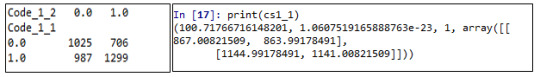
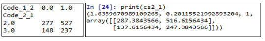
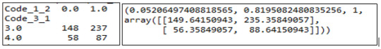
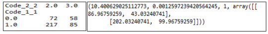
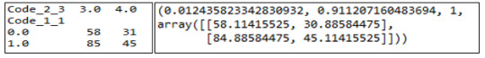
By looking at the above pictures we can say degree of freedom for all the combination is 1, We have also observed that p value for image 1 and 4 is less than .05, hence we will be accepting the alternate hypothesis and we can say there is association between people who interact very less or everyday they only do their homework properly.

Note : 0= never, 1= just a few times, 2= about once a week, 3= almost every day, 4= everyday

#coursera

0 notes

shadywolfclambiscuit-blog · 7 years ago

Text

Week 1: Hypothesis Testing and ANOVA

Used Dataset: ad_health

Hypothesis:

H0 (Null Hypothesis) = All age’s people are getting along with teacher do not have any difference in their mean

Ha (Alternative Hypothesis) = All age’s people are getting along with teacher have different mean

Selected Variable:

1- getting along with your teachers? (H1ED15) (Available Values are below)

0 - never

1 - just a few times

2 - about once a week

3 - almost everyday

4 - everyday

6 - refused

7 - legitimate skip

8 - don’t know

2- Age

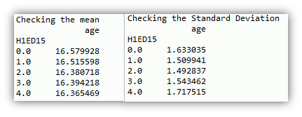
Model interpretation for ANOVA:

While evaluating the association between categorical variable “Getting along with your teachers? (H1ED15)” and quantitative variable “Age”. As categorical variable is having more than 2 values and we have also quantitative variable so we can go with the ANOVA. After running the ANOVA we have got below results. As we can see that p value is almost equal to .05(.049). Hence we accept the null hypothesis and conclude that there is no difference in mean of “Age” at different level of “Getting along with your teacher?”

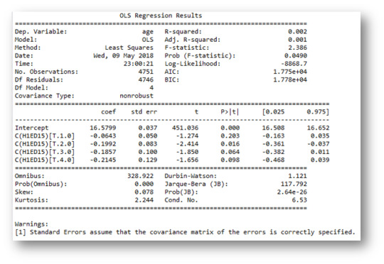
Also I have calculated mean and standard deviation separately to observe the difference between them and we can see there is minimal difference in there mean and standard deviation.

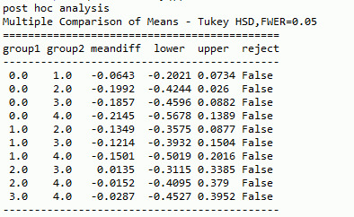
Model interpretation for post hoc ANOVA:

Below is the result from post hoc ANOVA, to run the post hoc for ANOVA I will be considering Tukey HSD method. There is none of the group available which shows that we can reject the null hypothesis. Now statistically we can say there is not significantly difference in means of different combination.

********************************Code********************************

# -*- coding: utf-8 -*- """ Created on Tue May 8 17:19:59 2018

@author: Nikhil Tripathi """

# importing the package

import pandas import numpy import statsmodels.formula.api as smf import statsmodels.stats.multicomp as ssm

""" Hypothesis : H0 = All age people are getting along with teacher do not have any difference in their mean Ha = All age people are getting along with teacher have different mean """

# loading the useful data

mydata = pandas.read_csv('Addhealth_pds.csv',low_memory = False) print(mydata.head(10))

# Creating a subset with required column mydata1 = mydata[['H1ED15','age']] print (mydata1.head(10))

# converting the data into numeric mydata1['H1ED15'] = mydata1['H1ED15'].convert_objects(convert_numeric=True) mydata1['age'] = mydata1['age'].convert_objects(convert_numeric=True)

# To check the summary count of the selected column c = mydata1['H1ED15'].value_counts(sort = True, dropna = False) print(c)

#Combing other values i.e. refused(6), don't know(8) and NaN into NaN mydata1['H1ED15'] = mydata1['H1ED15'].replace((6,7,8),numpy.nan) c = mydata1['H1ED15'].value_counts(sort = True, dropna = False) print(c)

# Checking Mean and Std (Standard Deviation) of the variable age print('Checking the mean') m1= mydata1.groupby('H1ED15').mean() print(m1)

print('Checking the Standard Deviation') m1= mydata1.groupby('H1ED15').std() print(m1)

# Now creating a subset without null value (excluding na) mydata2 = mydata1.dropna() print(mydata2.head(10))

# with the use of ols(ordinary least square) function calculating the F-Statistics and associated p value model1 = smf.ols(formula='age ~ C(H1ED15)', data=mydata2).fit() print (model1.summary())

# applying post hoc analysis and using the Tukey method for that print('post hoc analysis') mc1 = ssm.MultiComparison(mydata2['age'], mydata2['H1ED15']) res1 = mc1.tukeyhsd() print(res1.summary())

#coursera #python #anova

0 notes

shadywolfclambiscuit-blog · 7 years ago

Text

Week 4: Data Visualization Assignment

Code:

# -*- coding: utf-8 -*-

"""

Created on Fri Apr 28 19:47:39 2018

@author: Nikhil Tripathi

"""

#importing all the required packages

import pandas

import numpy

import seaborn

import matplotlib.pyplot as plt

#Reading Data file

mydata = pandas.read_csv('Addhealth_pds.csv',low_memory = False)

#setting pandas to show all the columns and row

pandas.set_option('display.max_columns', None)

pandas.set_option('display.max_rows', None)

# bug fix for display formats to avoid run time errors

pandas.set_option('display.float_format', lambda x:'%f'%x)

#Subsetting the data with required columns only and will be considering all the rows

mydata1 = mydata[['H1ED2', 'H1ED7', 'H1ED9', 'H1ED15', 'H1ED16', 'H1ED17', 'H1ED18', 'age']]

print(mydata1.head(10))

#Holding the subset data into new data frame

my_s_data = mydata1.copy()

#Converting metrics into numeric

my_s_data['H1ED2'] = my_s_data['H1ED2'].convert_objects(convert_numeric = True)

my_s_data['H1ED7'] = my_s_data['H1ED7'].convert_objects(convert_numeric = True)

my_s_data['H1ED9'] = my_s_data['H1ED9'].convert_objects(convert_numeric = True)

my_s_data['H1ED15'] = my_s_data['H1ED15'].convert_objects(convert_numeric = True)

my_s_data['H1ED16'] = my_s_data['H1ED16'].convert_objects(convert_numeric = True)

my_s_data['H1ED17'] = my_s_data['H1ED17'].convert_objects(convert_numeric = True)

my_s_data['H1ED18'] = my_s_data['H1ED18'].convert_objects(convert_numeric = True)

my_s_data['age'] = my_s_data['age'].convert_objects(convert_numeric = True)

#Missing Value Treatment and converting other values in single codes

print('After recoding 6 and 8 to nan')

my_s_data['c_sd'] = my_s_data['H1ED7'].replace((6,8), numpy.nan)

c_sd = my_s_data['c_sd'].fillna(101,inplace = True)

c = my_s_data['c_sd'].value_counts(dropna = False)

print(c)

#Creating this as first univariate chart for categorical variable

#To create this first we need to convert c_sd into categorical vaiable from numric

my_s_data['c_sd'] = my_s_data['c_sd'].astype('category')

seaborn.countplot(x='c_sd', data=my_s_data)

plt.xlabel('Responses from Participants')

plt.ylabel('Count of Participants')

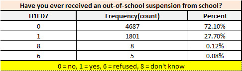
plt.title('Have you ever received an out-of-school suspension from school?')

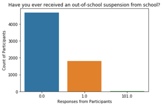
*********************Summary & Insights*********************

To get the above graph we have to do data preparation first like choosing the variable, convert any numeric field to category so it can be displayed properly. It’s type of Univariate chart.

Ø Legends (0 = no, 1 = yes, 101= unknown)

Ø Almost everyone is participated in the questioner and there is very minimal % of unknown

Ø We can see there is significant high numbers for the participants who did not received an out of school

Code:

#Univariate Histogram for Quantitate variable

seaborn.distplot(my_s_data['age'].dropna(), kde=False);

plt.title('Participants distribution in different Age group')

plt.ylabel('Total participants')

plt.xlabel('Age Group')

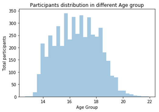
*********************Summary & Insights*********************

Ø To see the shape , range and spread of the data we have plotted a histogram

Ø Histogram shows that our data is unimodal

Ø We can observe that data is being normally distributed between the age range and there is none kind skewness in the data we can also run the descriptive Statistics on it to see the central tendency of the data

Code:

## Let's see the descriptive Stats for the Age metrics

# Which includes Min, Max, Stdv, Mean, median, mode

desc_age = my_s_data['age'].describe()

print('Describe the Age metrics')

print(desc_age)

## Descriptive stats can be seen by writting individual codes

print('Mean')

s_mean = my_s_data['age'].mean()

print(s_mean)

print('Mode')

s_mode = my_s_data['age'].mode()

print(s_mode)

print('Median')

s_median = my_s_data['age'].median()

print(s_median)

print('Min')

s_min = my_s_data['age'].min()

print(s_min)

print('Max')

s_max = my_s_data['age'].max()

print(s_max)

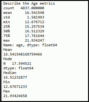
*********************Summary & Insights*********************

Ø There are two ways to describe the data mean to know about the its range, central tendency and spread of the data

Ø As we know if the data is normally distributed then mean ~ median ~ mode here we can see there is mean, median and mode are almost equal, it mean data is normal distributed and there is no outlier value available

Ø Also standard deviation is not high

Ø Hence we can say Age variable can be used for further analysis and it is normally distributed

Code:

## Creating Age categories

my_s_data['Age Catg.'] = pandas.cut(my_s_data.age,[0,14,18,22,26])

print('Age Catg.')

print(my_s_data['Age Catg.'])

#Converting this into category

my_s_data['Age Catg.'] = my_s_data['Age Catg.'].astype('category')

# Creating bivariate chart

seaborn.factorplot(x='Age Catg.', y='age', data=my_s_data, kind="bar", ci=None)

plt.xlabel('Age Categories group')

plt.ylabel('Age')

print('Age Distribution in various category')

# To make the categories more meaningful we can assign proper naming convention to them

# As that variable has already converted so we can use it else we have to convert it from numeric to categorical

my_s_data['Age Catg.'] = my_s_data['Age Catg.'].cat.rename_categories(['<14','14 to 18','19 to 22','22+'])

seaborn.factorplot(x='Age Catg.', y='age', data=my_s_data, kind="bar", ci=None)

plt.xlabel('Age Categories group')

plt.ylabel('Age')

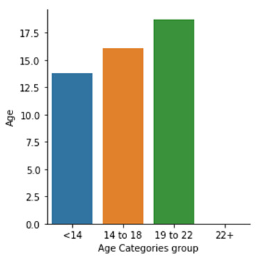
*********************Summary & Insights*********************

Ø Here we can see we have assigned logical names to the Age group

Ø We can see participants between Age group of 19 to 22 is significant higher than other age group

Code:

## Considering Gapminder data sets to plot some other type of graphs

import pandas

import numpy

import seaborn

import matplotlib.pyplot as plt

# Reading the gapminder data file

gm_data = pandas.read_csv('Gapminder.csv')

print (gm_data.head(10))

# Let's check number columns and row

print (len(gm_data))

print (len(gm_data.columns))

#Converting columns into numeric

gm_data['incomeperperson'] = gm_data['incomeperperson'].convert_objects(convert_numeric = True)

gm_data['alcconsumption'] = gm_data['alcconsumption'].convert_objects(convert_numeric = True)

gm_data['co2emissions'] = gm_data['co2emissions'].convert_objects(convert_numeric = True)

gm_data['oilperperson'] = gm_data['oilperperson'].convert_objects(convert_numeric = True)

# We can also describe the each and every column to see the spread of the data

gm_data['incomeperperson'].describe()

gm_data['alcconsumption'].describe()

gm_data['co2emissions'].describe()

gm_data['oilperperson'].describe()

#Let's find out the association Q->Q

#Creating Scatter plots Type 1 = Basic Scatter Plot

sctr_plt1 = seaborn.regplot(x = 'incomeperperson', y = 'alcconsumption', fit_reg = False , data = gm_data)

plt.xlabel('Income per person')

plt.ylabel('Alchohol Consumption')

plt.title('Association of Income per person with Alchohol Consumption')

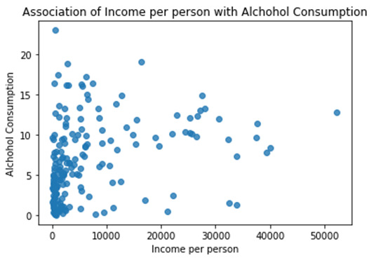
*********************Summary & Insights*********************

Ø To see the association between two measurable metrics we use Scatter plot

Ø Here we can see there is no significant association between Income per person and Alcohol consumption

Ø To understand the more about association we can use the fit line within the scatter plot which can be seen in the below upcoming scatter plot

Code:

#Creating scatter plots Type 2 = Includiing Regression fit line

sctr_plt2 = seaborn.regplot(x = 'incomeperperson', y = 'co2emissions', fit_reg = True, data = gm_data)

plt.xlabel('Income per preson')

plt.ylabel('Co2 emissions')

plt.title('Association of Income per person with Co2 emissions')

# As Type 2 gives us more information so we will be creating 2 more scatter plots in same way

sctr_plt3 = seaborn.regplot(x='incomeperperson', y='oilperperson', fit_reg=True, data = gm_data)

plt.xlabel ('Income per person')

plt.ylabel ('Oil per person')

plt.title ('Association of Income per person with Oil per person')

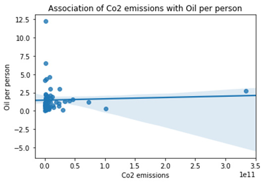
sctr_plt4 =seaborn.regplot(x= 'co2emissions', y= 'oilperperson', fit_reg=True, data = gm_data)

plt.xlabel ('Co2 emissions')

plt.ylabel ('Oil per person')

plt.title ('Association of Co2 emissions with Oil per person')

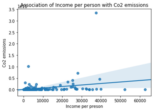
*********************Summary & Insights*********************

Ø By looking into the “'Association of Income per person with Co2 emissions” if we ignore couple of outlier value we can see association between these metrics and there is positive strong relationship mean one metrics is affective the other metrics, it show some way or other way Income per person is impacting the used of different things which could lead to generate more Co2 emissions.

Ø By looking into the “Association of Income per person with Oil per person” we can see there is weak positive relationship between the metrics and Income per person is impacting the Oil per person but not aggressively

Ø By looking into the “Association of Co2 emissions with Oil per person” we can see there is neutral association between both of the metrics it mean Co2 emissions and Oil per person is not impacting each other.

#coursera #python #graphs

0 notes

shadywolfclambiscuit-blog · 7 years ago

Text

Assignment 3 : Making Data Management Decisions

"""

Created on Wed Apr 18 18:13:21 2018

@author: Nikhil_Tripathi

"""

Assignment 3: Making Data Management Decisions

"""

#importing the packages

import pandas

import numpy

#Reading the data file in python for further analysis

mydata = pandas.read_csv('Addhealth_pds.csv',low_memory = False)

# Bug fix for display formats to avoid run time errors

pandas.set_option('display.float_format', lambda x:'%f'%x)

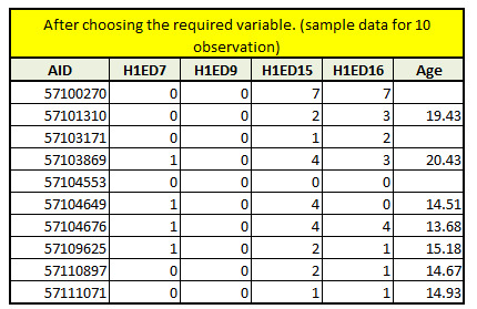
#getting only considerable variable in the dataframe by subsetting & choosing variable the data

sub_data1 = mydata[['AID', 'H1ED7', 'H1ED9', 'H1ED15', 'H1ED16','age']]

#coping the new dataframe which is subset of the mydata

sub_data = sub_data1.copy()

#checking the new subset of the data and to see if the only chosen variable is showing

print (sub_data.head (10))

#converting to numeric values and going forward in the below analysis we will be using subset which is sub_data

sub_data['H1ED7'] = sub_data['H1ED7'].convert_objects(convert_numeric = True)

sub_data['H1ED9'] = sub_data['H1ED9'].convert_objects(convert_numeric = True)

sub_data['H1ED15'] = sub_data['H1ED15'].convert_objects(convert_numeric = True)

sub_data['H1ED16'] = sub_data['H1ED16'].convert_objects(convert_numeric = True)

sub_data['age'] = sub_data['age'].convert_objects(convert_numeric = True)

#checking the Frequency (count) for the first variable H1ED7 with na values

# by assigning meaningful title

print('Have you ever received an out-of-school suspension from school?')

c_sd = sub_data['H1ED7'].value_counts(sort = False, dropna = False)

print(c_sd)

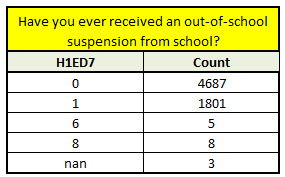
#As we have some nan values along with some values which can be considered nan for us like 6 and 8 which can be recoded

#0 = no, 1 = yes, 6 = refused, 8 = don't know

#recoding of the 6, 8 and nan to python missing (NaN)

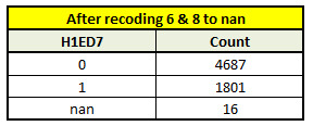
print('After recoding 6 and 8 to nan')

sub_data['H1ED7'] = sub_data['H1ED7'].replace((6,8), numpy.nan)

# Let's see how the recoding works, we should be able to see now 0, 1 and nan only because 6 & 8 is been recoded as nan

# We will see the frequency distribution again as we have done recoding, we have an option to drop nan value by making it dropna = True

print('After recoding 6 and 8 to nan, checking its impact on the data values')

c_sd = sub_data['H1ED7'].value_counts(sort = False, dropna = False)

print(c_sd)

# we can also assign a code to nan values, for example I would be assigning 101

print('Assigning a value to nan')

c_sd = sub_data['H1ED7'].fillna(101,inplace = True)

print(c_sd)

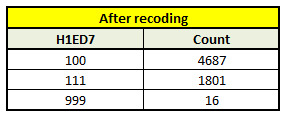
# recoding the values by creating new column

recode = {0: 100, 1: 111, 101: 999}

sub_data['new_variable'] = sub_data['H1ED7'].map(recode)

#Check how it impacts the subset and what kind of values is being recoded

#print(sub_data.head(25))

c_recode = sub_data['new_variable'].value_counts(sort = False)

print(c_recode)

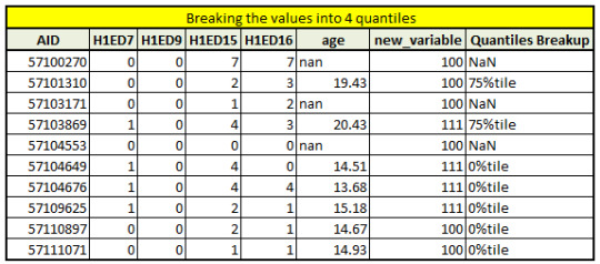
# To see the breakup at different quantiles we use qcut function

print ('Breaking the values into 4 quantiles')

sub_data['Quantiles Breakup'] = pandas.qcut(sub_data.age, 4 , labels=["0%tile","25%tile","50%tile","75%tile"],duplicates = 'drop')

print(sub_data.head(10))

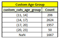
# creating categories by given splits value with the use of cut function

# splits into 4 groups (11-14, 14-17, 17-20, 20-23) - remember that Python starts counting from 0, not 1

sub_data['custom_cuts_age'] = pandas.cut(sub_data.age, [11, 14, 17, 20,23])

c5 = sub_data['custom_cuts_age'].value_counts(sort=False, dropna=False)

print(c5)

"""

Creating new variable, new variable can be create by using any existing field and available function

In this scenario I will be seeing how the two variables "Paying attention in school?" and "Getting your homework done?" Are related with each other by created a new variable which will be based on these 2 variables

"""

# First I am creating 3 categories which paying attention, not paying attention and no_answer for both of the variables

def H1ED16_new (row):

if row['H1ED16'] > 0 :

return 'paying attention'

if row['H1ED16'] == 0 :

return 'not paying attention'

sub_data['H1ED16_new'] = sub_data.apply (lambda row: H1ED16_new (row),axis=1)

print(sub_data.head(10))

# now we can also see the frequency of the new variable

c_new_var = sub_data['H1ED16_new'].value_counts(sort = False, dropna = False)

p_new_var = sub_data['H1ED16_new'].value_counts(sort = False, normalize = True)

print('Count & Percent')

print(c_new_var)

print(p_new_var)

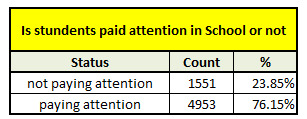
*****************Summary*******************************

Through this code I have got the opportunity to make manipulation with data by using Subset of the data with selected variable and using them further conversion of the data into meaningful data by recoding, assigning appropriate codes, working with null or nan fields. Also explored some of the functionality which allows me to create logical fields(additional field) with the help of existing field so we can generate more meaningful output.

By looking at the final output we can see there is significant % of students would like pay attention in the class.

#coursera

0 notes

shadywolfclambiscuit-blog · 7 years ago

Text

Week 2 Assignments- Writing your first program - Python

************************************Python Codes*************************************

""" Created on Fri Apr 13 17:10:53 2018

@author: Nikhil_Tripathi """

#To start with any analytical word in python we need to import the library/packages #In this case we will be importing "Pandas" and "Numpy' packages

#Importing library

import pandas import numpy

#After importing the library We have to get the required data for further analysis

#Reading the available .csv file and setting low_memory False so the efficiancy can be improved mydata = pandas.read_csv('Addhealth_pds.csv', low_memory= False)

#Counting number of available variable (columns in data file) print(len(mydata.columns))

#Getting count of total observations(Rows in the data file ) print(len(mydata))

#Converting all the variable as a numeric variable,so it will not be treated as String mydata['H1ED2'] = mydata['H1ED2'].convert_objects(convert_numeric = True) mydata['H1ED7'] = mydata['H1ED7'].convert_objects(convert_numeric = True) mydata['H1ED9'] = mydata['H1ED9'].convert_objects(convert_numeric = True) mydata['H1ED15'] = mydata['H1ED15'].convert_objects(convert_numeric = True) mydata['H1ED16'] = mydata['H1ED16'].convert_objects(convert_numeric = True) mydata['H1ED17'] = mydata['H1ED17'].convert_objects(convert_numeric = True) mydata['H1ED18'] = mydata['H1ED18'].convert_objects(convert_numeric = True) mydata['age'] = mydata['age'].convert_objects(convert_numeric = True)

#Check Frequency, which can be measured through Count and Percentage of the unique observation under each variable #Along with the tiles of the output so it will be easy to be identified print ('How many times {HAVE YOU SKIPPED/DID YOU SKIP} school for a full day without an excuse?') c1 = mydata['H1ED2'].value_counts(sort=True) p1 = mydata['H1ED2'].value_counts(sort=True, normalize=True) print (c1) print (p1)

print ('Have you ever received an out-of-school suspension from school?') c2 = mydata['H1ED7'].value_counts(sort=True) p2 = mydata['H1ED7'].value_counts(sort=True, normalize=True) print (c2) print (p2)

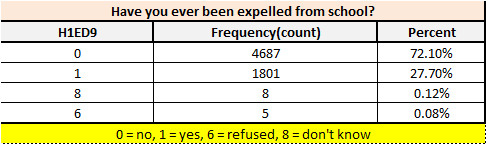
print ('Have you ever been expelled from school?') c3 = mydata['H1ED9'].value_counts(sort=True) p3 = mydata['H1ED9'].value_counts(sort=True, normalize=True) print (c3) print (p3)

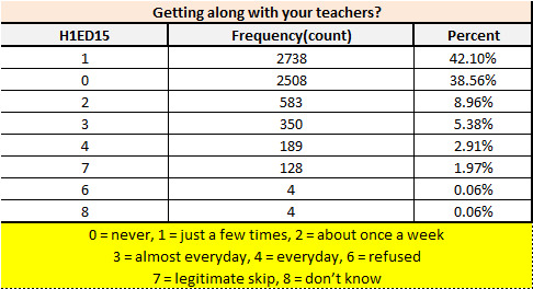
print ('Getting along with your teachers?') c4 = mydata['H1ED15'].value_counts(sort=True) p4 = mydata['H1ED15'].value_counts(sort=True, normalize=True) print (c4) print (p4)

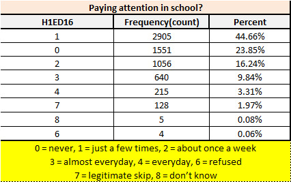
print ('Paying attention in school?') c5 = mydata['H1ED16'].value_counts(sort=True) p5 = mydata['H1ED16'].value_counts(sort=True, normalize=True) print (c5) print (p5)

print ('Getting your homework done?') c6 = mydata['H1ED17'].value_counts(sort=True) p6 = mydata['H1ED17'].value_counts(sort=True, normalize=True) print (c6) print (p6)

print ('Getting along with your teachers?') c7 = mydata['H1ED18'].value_counts(sort=True) p7 = mydata['H1ED18'].value_counts(sort=True, normalize=True) print (c7) print (p7)

print ('Age') c8 = mydata['H1ED18'].value_counts(sort=True) p8 = mydata['H1ED18'].value_counts(sort=True, normalize=True) print (c8) print (p8)

""" Another way of doing the above task(Frequency Distribution) with the use of Groupby function.(Frequency Distribution) """ ac1 = mydata.groupby('H1ED2').size() print(ac1)

#subset the data into 2 parts based on the given age less than 18 and greater than and equal to 18 age_less_18= mydata[(mydata['age']<18)] age_grt_18= mydata[(mydata['age']>=18)] #Checking Number of columns and Observation print(len(age_less_18)) print(len(age_less_18.columns))

#Holding subsetted data mydata_les_18 = age_less_18.copy() mydata_grt_18 = age_grt_18.copy()

#Now we can again see frequency distribution print ('Age <18,How many times {HAVE YOU SKIPPED/DID YOU SKIP} school for a full day without an excuse?')

c_les18 = mydata_les_18['H1ED2'].value_counts(sort=True) p_les18 = mydata_les_18['H1ED2'].value_counts(sort=True, normalize=True) print (c_les18) print (p_les18)

print ('Age >=18,How many times {HAVE YOU SKIPPED/DID YOU SKIP} school for a full day without an excuse?')

c_grt18 = mydata_grt_18['H1ED2'].value_counts(sort=True) p_grt18 = mydata_grt_18['H1ED2'].value_counts(sort=True, normalize=True) print (c_grt18) print (p_grt18)

#Turning all columns into upper case after loading data into python mydata.columns = map(str.upper, mydata.columns)

# bug fixing for display formats to avoid run time errors pandas.set_option('display.float_format', lambda x:'%f'%x)

++++++++++++++++++++++++++++++++++++++++++++++++++++++++++

+++++++Output (used Excel to format the python output)+++++++++++++++++

++++++++++++++++++++++++++++++++++++++++++++++++++++++++++

++++++++++++Summary Key Observations+++++++++++++++++++++++++++

For the analysis Add_Health data has been considered and there are total number of observations(rows) are 6504.

> For the first question "Have you ever received an out-of-school suspension from school?” We have observed that there is significant high number (72%) for "No Suspension" and there is very few people which refused/don't know (.20%) about the question. While doing the further analysis we can ignore them as well and we have good number of responses which will help us to drive some conclusion out of it.

> For the second question "Have you ever been expelled from school?", We have observed that there is significant high number(72%) for "Not expelled from school “and also we can also assume it is directly correlated with the first question which we can test later on.

> For the third question "Getting along with your teachers?” There is only 60% population has trouble with their teacher during their academic time, however there is 39% population which did not have any trouble with their teacher.

> For the fourth question “Paying attention in school?” There is major population falls in category of “Yes” they paid attention in school.

#coursera #myfisrtprograme #python

0 notes

shadywolfclambiscuit-blog · 7 years ago

Text

Week 1 – Assignment Getting Your Research Project Started

Week 1 – Assignment

Selecting the datasets:

As this is my first assignment on Coursera and specially with this course, so I am trying to do my best but still giving feedback will help me to grow more in upcoming days.

I have gone through all the 5 datasets and it was really tough to select a dataset which I will be using for further my analysis. However By looking into the variables and Unit of observation I found my interest in “AddHealth” datasets as It is belongs to my teen age and I am able to relate most of the variable with my real experience.

It has lot of information with available data variable in different sections. Out of all the section I would be going with “Section 5: Academics and Education” and picking up right codebook for my work.

Research Question:

How Academics and Education play a great role in the Adolescents and understand what kind variable (Related with education) impact the individual personality.

Hypothesis:

§ Is receiving out-of-school suspension define the individual personality

§ Is getting home-work done shows the disciplined of the person

§ What is the correlation between being happy from beginning to end of the school and its impacting the individual

§ Is repeating a grade is defining the individual

Selection of Variables:

Although there are so many variables available under the above mentioned section (Section 5) but to run my hypothesis I would prefer to use relevant variable, However I will never mind to utilize my time and run the instant hypothesis on other variables too. I have included variable names at the last.

Search Term Used to get more information about the Research Question:

Ø Academic and Education on adolescents

Ø Impact of Education and Academy on Adolescent

Ø School Environment And Adolescent

Reference Links:

I would like to put some of the sources URL, which I have referred while reading more about the research question.

1. Citation: Through this we can understand how we can get more efficacies of Adolescents by looking into different aspects of the real life behaviors and by changing some of the habits can make significant difference in adolescents. Some of the Key things are :

· A Social Cognitive Perspective

· Too much confidence and learning Disabilities

· Implications for Teachers and Parents

· Factors Influencing Academic Achievement in Collectivist Societies

Refer this URL: https://www.uky.edu/~eushe2/Pajares/AdoEd5.html

2. Citation: A survey had been conducted where 100 people participated from various groups of society. Survey was having good questioner which may help us to read their personal behavior and thought process, which will help us to understand the data pretty well and how those numbers have been derived. Some of the Key Questions are:

· Ability to get things done and to work smoothly with others

· Self-motivation .to learn, participate, achieve

· Problem solving

· Risk taking--being assertive and independent

Refer this URL: https://digitalcommons.unomaha.edu/cgi/viewcontent.cgi?article=1006&context=slcek12

3. Citation: I found this good research paper; it includes lots of stats about different Age groups and some other attributes. There are some good points are:

· Schools Safety and Violence

· Schools and Health Care

· Academic Quality

· Schools and Obesity

Refer this URL: https://www.childtrends.org/wp-content/uploads/2013/04/child_trends-2008_11_14_rb_schoolenviron.pdf

Summary: By Looking in the existing data variable and other references(which are above mentioned), I am able to get some good points which can be consider while finding out the significance correlation of the Academic and Education on adolescent. Few of the findings and take away which I will be utilizing throughout the learning.

Ø If a person is involve in any kind of bad things during school time that person will be having high chance to be unhappy while leaving the school

Ø How’s Teachers qualification and Parent’s behavior help the children to be happy in their schooling which directly positively impact in their adolescents

Ø Self-confidence of the person will also help them to be happy and also participates in school activities , which also positively impact their adolescents

Ø More finding can be stated here after testing the hypothesis J

--------------------------------------------------------------------------------------------------------------------------------------------

Used Variables:

Section 5: Academics and Education

1. [If SCHOOL YEAR:] During this school year how many times {HAVE YOU} . . . . . . . . . . . . H1ED1

YOU BEEN/WERE YOU} absent from school for a full day with an excuse—for

example, because you were sick or out of town?

[If SUMMER:] During the 1994-1995 school year how many times {HAVE YOU BEEN/WERE

YOU} absent from school for a full day with an excuse—for

example, because you were sick or out of town?

2. [If SCHOOL YEAR:] During this school year how many times {HAVE YOU . . . . . . . . . . . . H1ED2

SKIPPED/DID YOU SKIP} school for a full day without an excuse?

[If SUMMER:] During the 1994-1995 school year how many times {HAVE YOU

SKIPPED/DID YOU SKIP} school for a full day without an excuse?

3. Have you ever skipped a grade? . . . . . . . . . . . . . . . . . . . . . . . . . . . . . . . . . . . . . . . . . . . . . . . . . . H1ED3

4. Which grades have you skipped?

first . . . . . . . . . . . . . . . . . . . . . . . . . . . . . . . . . . . . . . . . . . . . . . . . . . . . . . . . . . . . . . . . . . . . . . . H1ED4A

second . . . . . . . . . . . . . . . . . . . . . . . . . . . . . . . . . . . . . . . . . . . . . . . . . . . . . . . . . . . . . . . . . . . . . H1ED4B

third . . . . . . . . . . . . . . . . . . . . . . . . . . . . . . . . . . . . . . . . . . . . . . . . . . . . . . . . . . . . . . . . . . . . . . . H1ED4C

fourth . . . . . . . . . . . . . . . . . . . . . . . . . . . . . . . . . . . . . . . . . . . . . . . . . . . . . . . . . . . . . . . . . . . . . . H1ED4D

fifth . . . . . . . . . . . . . . . . . . . . . . . . . . . . . . . . . . . . . . . . . . . . . . . . . . . . . . . . . . . . . . . . . . . . . . . H1ED4E

sixth . . . . . . . . . . . . . . . . . . . . . . . . . . . . . . . . . . . . . . . . . . . . . . . . . . . . . . . . . . . . . . . . . . . . . . . H1ED4F

seventh . . . . . . . . . . . . . . . . . . . . . . . . . . . . . . . . . . . . . . . . . . . . . . . . . . . . . . . . . . . . . . . . . . . . . H1ED4G

eighth . . . . . . . . . . . . . . . . . . . . . . . . . . . . . . . . . . . . . . . . . . . . . . . . . . . . . . . . . . . . . . . . . . . . . . H1ED4H

ninth . . . . . . . . . . . . . . . . . . . . . . . . . . . . . . . . . . . . . . . . . . . . . . . . . . . . . . . . . . . . . . . . . . . . . . . H1ED4I

tenth . . . . . . . . . . . . . . . . . . . . . . . . . . . . . . . . . . . . . . . . . . . . . . . . . . . . . . . . . . . . . . . . . . . . . . . . H1ED4J

eleventh . . . . . . . . . . . . . . . . . . . . . . . . . . . . . . . . . . . . . . . . . . . . . . . . . . . . . . . . . . . . . . . . . . . . H1ED4K

school not graded . . . . . . . . . . . . . . . . . . . . . . . . . . . . . . . . . . . . . . . . . . . . . . . . . . . . . . . . . . . H1ED4M

5. Have you ever repeated a grade or been held back a grade? . . . . . . . . . . . . . . . . . . . . . . . . . . . . H1ED5

In Home Questionnaire Code Book

Questions and Variable Names

Question Variable Name

6. Which grades have you repeated?

first . . . . . . . . . . . . . . . . . . . . . . . . . . . . . . . . . . . . . . . . . . . . . . . . . . . . . . . . . . . . . . . . . . . . . . . H1ED6A

second . . . . . . . . . . . . . . . . . . . . . . . . . . . . . . . . . . . . . . . . . . . . . . . . . . . . . . . . . . . . . . . . . . . . . H1ED6B

third . . . . . . . . . . . . . . . . . . . . . . . . . . . . . . . . . . . . . . . . . . . . . . . . . . . . . . . . . . . . . . . . . . . . . . . H1ED6C

fourth . . . . . . . . . . . . . . . . . . . . . . . . . . . . . . . . . . . . . . . . . . . . . . . . . . . . . . . . . . . . . . . . . . . . . . H1ED6D

fifth . . . . . . . . . . . . . . . . . . . . . . . . . . . . . . . . . . . . . . . . . . . . . . . . . . . . . . . . . . . . . . . . . . . . . . . H1ED6E

sixth . . . . . . . . . . . . . . . . . . . . . . . . . . . . . . . . . . . . . . . . . . . . . . . . . . . . . . . . . . . . . . . . . . . . . . . H1ED6F

seventh . . . . . . . . . . . . . . . . . . . . . . . . . . . . . . . . . . . . . . . . . . . . . . . . . . . . . . . . . . . . . . . . . . . . . H1ED6G

eighth . . . . . . . . . . . . . . . . . . . . . . . . . . . . . . . . . . . . . . . . . . . . . . . . . . . . . . . . . . . . . . . . . . . . . . H1ED6H

ninth . . . . . . . . . . . . . . . . . . . . . . . . . . . . . . . . . . . . . . . . . . . . . . . . . . . . . . . . . . . . . . . . . . . . . . . H1ED6I

tenth . . . . . . . . . . . . . . . . . . . . . . . . . . . . . . . . . . . . . . . . . . . . . . . . . . . . . . . . . . . . . . . . . . . . . . . . H1ED6J

eleventh . . . . . . . . . . . . . . . . . . . . . . . . . . . . . . . . . . . . . . . . . . . . . . . . . . . . . . . . . . . . . . . . . . . . H1ED6K

twelfth . . . . . . . . . . . . . . . . . . . . . . . . . . . . . . . . . . . . . . . . . . . . . . . . . . . . . . . . . . . . . . . . . . . . . H1ED6L

school not graded . . . . . . . . . . . . . . . . . . . . . . . . . . . . . . . . . . . . . . . . . . . . . . . . . . . . . . . . . . . H1ED6M

7. Have you ever received an out-of-school suspension from school? . . . . . . . . . . . . . . . . . . . . . . H1ED7

8. What grade were you in the last time this happened? . . . . . . . . . . . . . . . . . . . . . . . . . . . . . . . . . H1ED8

9. Have you ever been expelled from school? . . . . . . . . . . . . . . . . . . . . . . . . . . . . . . . . . . . . . . . . . H1ED9

10. What grade were you in the last time this happened? . . . . . . . . . . . . . . . . . . . . . . . . . . . . . . . . . H1ED10

11. At the {MOST RECENT GRADING PERIOD/LAST GRADING PERIOD IN . . . . . . . . H1ED11

THE SPRING}, what was your grade in English or language arts?

12. And what was your grade in mathematics? . . . . . . . . . . . . . . . . . . . . . . . . . . . . . . . . . . . . . . . . . H1ED12

13. And what was your grade in history or social studies? . . . . . . . . . . . . . . . . . . . . . . . . . . . . . . . . . H1ED13

14. And what was your grade in science? . . . . . . . . . . . . . . . . . . . . . . . . . . . . . . . . . . . . . . . . . . . . . . H1ED14

[If SCHOOL YEAR:] Since school started this year, how often have you had trouble:

[If SUMMER:] During the 1994-1995 school year, how often did you have trouble:

15. getting along with your teachers? . . . . . . . . . . . . . . . . . . . . . . . . . . . . . . . . . . . . . . . . . . . . . . . . . H1ED15

16. paying attention in school? . . . . . . . . . . . . . . . . . . . . . . . . . . . . . . . . . . . . . . . . . . . . . . . . . . . . . . H1ED16

17. getting your homework done? . . . . . . . . . . . . . . . . . . . . . . . . . . . . . . . . . . . . . . . . . . . . . . . . . . . H1ED17

18. getting along with other students? . . . . . . . . . . . . . . . . . . . . . . . . . . . . . . . . . . . . . . . . . . . . . . . . H1ED18

19. [If SCHOOL YEAR:] You feel close to people at your school. . . . . . . . . . . . . . . . . . . . . . . . . . H1ED19

[If SUMMER:] Last year, you felt close to people at your school.

20. [If SCHOOL YEAR:] You feel like you are part of your school. . . . . . . . . . . . . . . . . . . . . . . . H1ED20

[If SUMMER:] Last year, you felt like you were part of your school.

21. [If SCHOOL YEAR:] Students at your school are prejudiced. . . . . . . . . . . . . . . . . . . . . . . . . . . H1ED21

[If SUMMER:] Last year, the students at your school were prejudiced.

22. [If SCHOOL YEAR:] You are happy to be at your school. . . . . . . . . . . . . . . . . . . . . . . . . . . . H1ED22

[If SUMMER:] Last year, you were happy to be at your school.

23. [If SCHOOL YEAR:] The teachers at your school treat students fairly. . . . . . . . . . . . . . . . . . H1ED23

[If SUMMER:] Last year, the teachers at your school treated students fairly.

24. [If SCHOOL YEAR:] You feel safe in your school. . . . . . . . . . . . . . . . . . . . . . . . . . . . . . . . . . H1ED24

[If SUMMER:] Last year, you felt safe in your school.

#coursera #1st_assignment #journeybegins

0 notes

shadywolfclambiscuit-blog · 7 years ago

Text

#MyProject

Week 1 – Assignment

Selecting the datasets:

As this is my first assignment on Coursera and specially with this course, so I am trying to do my best but still giving feedback will help me to grow more in upcoming days.

Research Question:

How Academics and Education play a great role in the Adolescents and understand what kind variable (Related with education) impact the individual personality.

Hypothesis:

§ Is receiving out-of-school suspension define the individual personality

§ Is getting home-work done shows the disciplined of the person

§ What is the correlation between being happy from beginning to end of the school and its impacting the individual

§ Is repeating a grade is defining the individual

Selection of Variables:

References:

I would like to put some of the sources URL, which I have referred while reading more about the research question.

1. https://www.uky.edu/~eushe2/Pajares/AdoEd5.html

2. https://digitalcommons.unomaha.edu/cgi/viewcontent.cgi?article=1006&context=slcek12

3. https://www.childtrends.org/wp-content/uploads/2013/04/child_trends-2008_11_14_rb_schoolenviron.pdf

4. https://pdfs.semanticscholar.org/a17a/896532fba4e54aff126537014c4e5429c343.pdf