#43093 | Explore Tumblr Posts and Blogs

dataanalyst75 · 2 months

Text

Running a Lasso Regression Analysis to identify a subset of variables that best predicted the alcohol drinking behavior of individuals

A lasso regression analysis is performed to detect a subgroup of variables from a set of 23 categorical and quantitative predictor variables in the Nesarc Wave 1 dataset which best predicted a quantitative response variable assessing the alcohol drinking behaviour of individuals 18 years and older in terms of number of any alcohol drunk per month.

Categorical predictors include a series of 5 binary categorical variables for ethnicity (Hispanic, White, Black, Native American and Asian) to improve interpretability of the selected model with fewer predictors.

Other binary categorical predictors are related to substance consumption, and in particular to the fact whether or not individuals are lifetime opioids, cannabis, cocaine, sedatives, tranquilizers consumers, as well as suffer from depression.

About dependencies, other binary categorical variables are those regarding if individuals

are lifetime affected by nicotine dependency,

abuse lifetime of alcohol

or not.

Quantitative predictor variables include age when the aforementioned substances have been taken for the first time, the usual frequency of cigarettes and of any alcohol drunk per month, the number of cigarettes smoked per month.

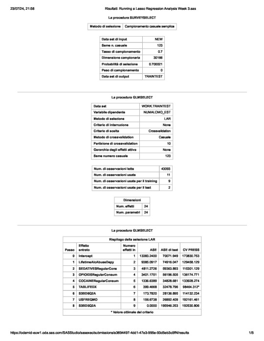
In a nutshell, looking at the SAS output,

the survey select procedure, used to split the observations in the dataset into training and test data, shows that the sample size is 30,166.

the so-called “NUMALCMO_EST” dependent variable - number of any alcohol drunk per month - along with the selection method used, are being displayed, together with information such as

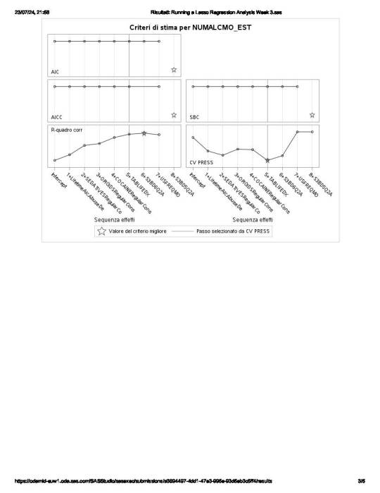
the choice of a cross validation criteria as criterion for choosing the best model, with K equals 10-fold cross validation,

the random assignments of observations to the folds

the total number of observations in the data set are 43093 and the number of observations used for training and testing the statistical models are 11, where 9 are for training and 2 for testing

the number of parameters to be estimated is 24 for the intercept plus the 23 predictors.

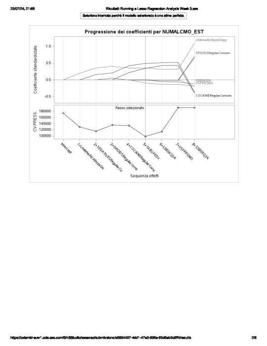
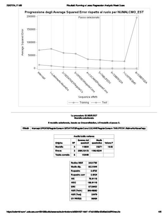
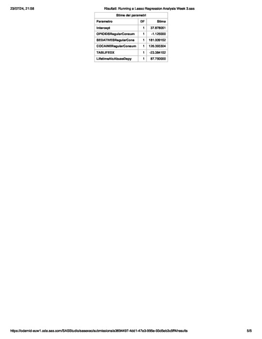
of the 23 predictor variables, 8 have been maintained in the selected model:

LifetimeAlcAbuseDepy - alcohol abuse / dependence both in last 12 months and prior to the last 12 months

and

OPIOIDSRegularConsumer – used opioids both in the last 12 months and prior to the last 12 months

have the largest regression coefficient, followed by COCAINERegularConsum behaviour.

LifetimeAlcAbuseDepy and OPIOIDSRegularConsum are positively associated with the response variable, while COCAINERegularConsum is negatively associated with NUMALCMO_EST.

Other predictors associated with lower number of any alcohol drunk per month are S3BD6Q2A – “age first used cocaine or crack” and USEFREQMO – “usual frequency of cigarettes smoked per month”.

These 8 variables accounted for 33.6% of the variance in the number of any alcohol drunk per month response variable.

Hereunder the SAS code used to generate the present analysis and the plots on which the above described results are depicted

PROC IMPORT DATAFILE ='/home/u63783903/my_courses/nesarc_pds.csv' OUT = imported REPLACE; RUN; DATA new; set imported;

/* lib name statement and data step to call in the NESARC data set for the purpose of growing decision trees*/

LABEL MAJORDEPLIFE = "MAJOR DEPRESSION - LIFETIME" ETHRACE2A = "IMPUTED RACE/ETHNICITY" WhiteGroup = "White, Not Hispanic or Latino" BlackGroup = "Black, Not Hispanic or Latino" NamericaGroup = "American Indian/Alaska Native, Not Hispanic or Latino" AsianGroup = "Asian/Native Hawaiian/Pacific Islander, Not Hispanic or Latino" HispanicGroup = "Hispanic or Latino" S3BD3Q2B = "USED OPIOIDS IN THE LAST 12 MONTHS/PRIOR TO LAST 12 MONTHS/BOTH TIME PERIODS" OPIOIDSRegularConsumer = "USED OPIOIDS both IN THE LAST 12 MONTHS AND PRIOR TO LAST 12 MONTHS" S3BD3Q2A = "AGE FIRST USED OPIOIDS" S3BD5Q2B = "USED CANNABIS IN THE LAST 12 MONTHS/PRIOR TO LAST 12 MONTHS/BOTH TIME PERIODS" CANNABISRegularConsumer = "USED CANNABIS both IN THE LAST 12 MONTHS AND PRIOR TO LAST 12 MONTHS" S3BD5Q2A = "AGE FIRST USED CANNABIS" S3BD1Q2B = "USED SEDATIVES IN THE LAST 12 MONTHS/PRIOR TO LAST 12 MONTHS/BOTH TIME PERIODS" SEDATIVESRegularConsumer = "USED SEDATIVES both IN THE LAST 12 MONTHS/PRIOR TO LAST 12 MONTHS" S3BD1Q2A = "AGE FIRST USED SEDATIVES" S3BD2Q2B = "USED TRANQUILIZERS IN THE LAST 12 MONTHS/PRIOR TO LAST 12 MONTHS/BOTH TIME PERIODS" TRANQUILIZERSRegularConsumer = "USED TRANQUILIZERS both IN THE LAST 12 MONTHS AND PRIOR TO LAST 12 MONTHS" S3BD2Q2A = "AGE FIRST USED TRANQUILIZERS" S3BD6Q2B = "USED COCAINE OR CRACK IN THE LAST 12 MONTHS/PRIOR TO LAST 12 MONTHS/BOTH TIME PERIODS" COCAINERegularConsumer = "USED COCAINE both IN THE LAST 12 MONTHS AND PRIOR TO LAST 12 MONTHS" S3BD6Q2A = "AGE FIRST USED COCAINE OR CRACK" TABLIFEDX = "NICOTINE DEPENDENCE - LIFETIME" ALCABDEP12DX = "ALCOHOL ABUSE/DEPENDENCE IN LAST 12 MONTHS" ALCABDEPP12DX = "ALCOHOL ABUSE/DEPENDENCE PRIOR TO THE LAST 12 MONTHS" LifetimeAlcAbuseDepy = "ALCOHOL ABUSE/DEPENDENCE both IN LAST 12 MONTHS and PRIOR TO THE LAST 12 MONTHS" S3AQ3C1 = "USUAL QUANTITY WHEN SMOKED CIGARETTES" S3AQ3B1 = "USUAL FREQUENCY WHEN SMOKED CIGARETTES" USFREQMO = "usual frequency of cigarettes smoked per month" NUMCIGMO_EST= "NUMBER OF cigarettes smoked per month" S2AQ8A = "HOW OFTEN DRANK ANY ALCOHOL IN LAST 12 MONTHS" S2AQ8B = "NUMBER OF DRINKS OF ANY ALCOHOL USUALLY CONSUMED ON DAYS WHEN DRANK ALCOHOL IN LAST 12 MONTHS" USFREQALCMO = "usual frequency of any alcohol drunk per month" NUMALCMO_EST = "NUMBER OF ANY ALCOHOL drunk per month" S3BD1Q2E = "HOW OFTEN USED SEDATIVES WHEN USING THE MOST" USFREQSEDATIVESMO = "usual frequency of any alcohol drunk per month" S1Q1F = "BORN IN UNITED STATES"

if cmiss(of _all_) then delete; /* delete observations with missing data on any of the variables in the NESARC dataset */

if ETHRACE2A=1 then WhiteGroup=1; else WhiteGroup=0; /* creation of a variable for white ethnicity coded for 0 for non white ethnicity and 1 for white ethnicity */

if ETHRACE2A=2 then BlackGroup=1; else BlackGroup=0; /* creation of a variable for black ethnicity coded for 0 for non black ethnicity and 1 for black ethnicity */

if ETHRACE2A=3 then NamericaGroup=1; else NamericaGrouGroup=0; /* same for native american ethnicity*/

if ETHRACE2A=4 then AsianGroup=1; else AsianGroup=0; /* same for asian ethnicity */

if ETHRACE2A=5 then HispanicGroup=1; else HispanicGroup=0; /* same for hispanic ethnicity */

if S3BD3Q2B = 9 then S3BD3Q2B = .; /* unknown observations set to missing data wrt usage of OPIOIDS IN THE LAST 12 MONTHS/PRIOR TO LAST 12 MONTHS/BOTH TIME PERIODS */

if S3BD3Q2B = 3 then OPIOIDSRegularConsumer = 1; if S3BD3Q2B = 1 or S3BD3Q2B = 2 then OPIOIDSRegularConsumer = 0; if S3BD3Q2B = . then OPIOIDSRegularConsumer = .; /* creation of a group variable where lifetime opioids consumers are coded to 1 and 0 for non lifetime opioids consumers */

if S3BD3Q2A = 99 then S3BD3Q2A = . ; /* unknown observations set to missing data wrt AGE FIRST USED OPIOIDS */

if S3BD5Q2B = 9 then S3BD5Q2B = .; /* unknown observations set to missing data wrt usage of CANNABIS IN THE LAST 12 MONTHS/PRIOR TO LAST 12 MONTHS/BOTH TIME PERIODS */

if S3BD5Q2B = 3 then CANNABISRegularConsumer = 1; if S3BD5Q2B = 1 or S3BD5Q2B = 2 then CANNABISRegularConsumer = 0; if S3BD5Q2B = . then CANNABISRegularConsumer = .; /* creation of a group variable where lifetime cannabis consumers are coded to 1 and 0 for non lifetime cannabis consumers */

if S3BD5Q2A = 99 then S3BD5Q2A = . ; /* unknown observations set to missing data wrt AGE FIRST USED CANNABIS */

if S3BD1Q2B = 9 then S3BD1Q2B = .; /* unknown observations set to missing data wrt usage of SEDATIVES IN THE LAST 12 MONTHS/PRIOR TO LAST 12 MONTHS/BOTH TIME PERIODS */

if S3BD1Q2B = 3 then SEDATIVESRegularConsumer = 1; if S3BD1Q2B = 1 or S3BD1Q2B = 2 then SEDATIVESRegularConsumer = 0; if S3BD1Q2B = . then SEDATIVESRegularConsumer = .; /* creation of a group variable where lifetime sedatives consumers are coded to 1 and 0 for non lifetime sedatives consumers */

if S3BD1Q2A = 99 then S3BD1Q2A = . ; /* unknown observations set to missing data wrt AGE FIRST USED sedatives */

if S3BD2Q2B = 9 then S3BD1Q2B = .; /* unknown observations set to missing data wrt usage of TRANQUILIZERS IN THE LAST 12 MONTHS/PRIOR TO LAST 12 MONTHS/BOTH TIME PERIODS */

if S3BD2Q2B = 3 then TRANQUILIZERSRegularConsumer = 1; if S3BD2Q2B = 1 or S3BD2Q2B = 2 then TRANQUILIZERSRegularConsumer = 0; if S3BD2Q2B = . then TRANQUILIZERSRegularConsumer = .; /* creation of a group variable where lifetime TRANQUILIZERS consumers are coded to 1 and 0 for non lifetime TRANQUILIZERS consumers */

if S3BD2Q2A = 99 then S3BD2Q2A = . ; /* unknown observations set to missing data wrt AGE FIRST USED TRANQUILIZERS */

if S3BD6Q2A = 9 then S3BD6Q2A = .; /* unknown observations set to missing data wrt usage of COCAINE IN THE LAST 12 MONTHS/PRIOR TO LAST 12 MONTHS/BOTH TIME PERIODS */

if S3BD6Q2B = 3 then COCAINERegularConsumer = 1; if S3BD6Q2B = 1 or S3BD6Q2B = 2 then COCAINERegularConsumer = 0; if S3BD6Q2B = . then COCAINERegularConsumer = .; /* creation of a group variable where lifetime COCAINE consumers are coded to 1 and 0 for non lifetime COCAINE consumers */

if S3BD6Q2A = 99 then S3BD2Q2A = . ; /* unknown observations set to missing data wrt AGE FIRST USED COCAINE */

if ALCABDEP12DX = 3 and ALCABDEPP12DX = 3 then LifetimeAlcAbuseDepy =1; else LifetimeAlcAbuseDepy = 0; /* creation of a group variable where consumers with lifetime alcohol abuse and dependence are coded to 1 and 0 for consumers with no lifetime alcohol abuse and dependence */

if S3AQ3C1=99 THEN S3AQ3C1=.;

IF S3AQ3B1=9 THEN SS3AQ3B1=.;

IF S3AQ3B1=1 THEN USFREQMO=30; ELSE IF S3AQ3B1=2 THEN USFREQMO=22; ELSE IF S3AQ3B1=3 THEN USFREQMO=14; ELSE IF S3AQ3B1=4 THEN USFREQMO=5; ELSE IF S3AQ3B1=5 THEN USFREQMO=2.5; ELSE IF S3AQ3B1=6 THEN USFREQMO=1; /* usual frequency of smoking per month */

NUMCIGMO_EST=USFREQMO*S3AQ3C1; /* number of cigarettes smoked per month */

if S2AQ8A=99 THEN S2AQ8A=.;

if S2AQ8B = 99 then S2AQ8B = . ;

IF S2AQ8A=1 THEN USFREQALCMO=30; ELSE IF S2AQ8A=2 THEN USFREQALCMO=30; ELSE IF S2AQ8A=3 THEN USFREQALCMO=14; ELSE IF S2AQ8A=4 THEN USFREQALCMO=8; ELSE IF S2AQ8A=5 THEN USFREQALCMO=4; ELSE IF S2AQ8A=6 THEN USFREQALCMO=2.5; ELSE IF S2AQ8A=7 THEN USFREQALCMO=1; ELSE IF S2AQ8A=8 THEN USFREQALCMO=0.75; ELSE IF S2AQ8A=9 THEN USFREQALCMO=0.375; ELSE IF S2AQ8A=10 THEN USFREQALCMO=0.125; /* usual frquency of alcohol drinking per month */

NUMALCMO_EST=USFREQALCMO*S2AQ8B; /* number of any alcohol drunk per month */

if S3BD1Q2E=99 THEN S3BD1Q2E=.;

IF S3BD1Q2E=1 THEN USFREQSEDATIVESMO=30; ELSE IF S3BD1Q2E=2 THEN USFREQSEDATIVESMO=30; ELSE IF S3BD1Q2E=3 THEN USFREQSEDATIVESMO=14; ELSE IF S3BD1Q2E=4 THEN USFREQSEDATIVESMO=6; ELSE IF S3BD1Q2E=5 THEN USFREQSEDATIVESMO=2.5; ELSE IF S3BD1Q2E=6 THEN USFREQSEDATIVESMO=1; ELSE IF S3BD1Q2E=7 THEN USFREQSEDATIVESMO=0.75; ELSE IF S3BD1Q2E=8 THEN USFREQSEDATIVESMO=0.375; ELSE IF S3BD1Q2E=9 THEN USFREQSEDATIVESMO=0.17; ELSE IF S3BD1Q2E=10 THEN USFREQSEDATIVESMO=0.083; /* usual frequency of seadtives assumption per month */

run;

ods graphics on; /* ODS graphics turned on to manage the output and displays in HTML */

proc surveyselect data=new out=traintest seed = 123 samprate=0.7 method=srs outall; run;

/* split data randomly into training data consisting of 70% of the total observations () test dataset consisting of the other 30% of the observations respectively)*/ /* data=new specifies the name of the managed input data set */ /* out equals the name of the randomly split output dataset, called traintest */ /* seed option to specify a random number seed to ensure that the data are randomly split the same way if the code being run again */ /* samprate command split the input data set so that 70% of the observations are being designated as training observations (the remaining 30% are being designated as test observations respectively) */ /* method=srs specifies that the data are to be split using simple random sampling */ /* outall option includes, both the training and test observations in a single output dataset which has a new variable called "selected", to indicate if an observation belongs to the training set, or the test set */

proc glmselect data=traintest plots=all seed=123; partition ROLE=selected(train='1' test='0'); /* glmselect procedure to test the lasso multiple regression w/ Least Angled Regression algorithm k=10 fold validation glmselect procedure standardize the predictor variables, so that they all have a mean equal to 0 and a standard deviation equal to 1, which places them all on the same scale data=traintest to use the randomly split dataset plots=all option to require that all plots associated w/ the lasso regression being printed seed option to allow to specify a random number seed, being used in the cross-validation process partition command to assign each observation a role, based on the variable called selected, indicating if the observation is a training or test observation. Observations with a value of 1 on the selected variable are assigned the role of training observation (observations with a value of 0, are assigned the role of test observation respectively) */

model NUMALCMO_EST = MAJORDEPLIFE WhiteGroup BlackGroup NamericaGroup AsianGroup HispanicGroup OPIOIDSRegularConsumer S3BD3Q2A CANNABISRegularConsumer S3BD5Q2A SEDATIVESRegularConsumer S3BD1Q2A TRANQUILIZERSRegularConsumer S3BD2Q2A COCAINERegularConsumer S3BD6Q2A TABLIFEDX LifetimeAlcAbuseDepy USFREQMO NUMCIGMO_EST USFREQALCMO S3BD1Q2E USFREQSEDATIVESMO/selection=lar(choose=cv stop=none) cvmethod=random(10); /* model command to specify the regression model for which the response variable, NUMALCMO_EST, is equal to the list of the 14 candidate predictor variables */ /* selection option to tell which method to use to compute the parameters for variable selection */ /*Least Angled Regression algorithm is being used */ /* choose=cv option to use cross validation for choosing the final statistical model */ /* stop=none to guarantee the model doesn't stop running until each of the candidate predictor variables is being tested */ /* cvmethod=random(10) to specify a K-fold cross-validation method with ten randomly selected folds is being used */ run;

0 notes

perimichael · 3 months

Text

LIBNAME mydata "/courses/d1406ae5ba27fe300 " access=readonly; DATA new; set mydata.nesarc_pds;

IF S1Q6A eq 1 THEN incomegroup=.; ELSE IF S1Q6A LE 3 THEN education=1; ELSE IF S1Q6A LE 5 THEN education=2; ELSE IF S1Q6A LE 7 THEN education=3; ELSE IF S1Q6A GT 10 THEN education=3;

PROC SORT; by IDNUM;

PROC CORR; VAR S1Q10B S1Q11B;

RUN;

The CORR Procedure2 Variables:S1Q10B S1Q11BSimple StatisticsVariableNMeanStd DevSumMinimumMaximumS1Q10B430936.757504.40665291201017.00000S1Q11B430939.421414.843084059971.0000021.00000Pearson Correlation Coefficients, N = 43093 Prob > |r| under H0: Rho=0 S1Q10BS1Q11BS1Q10B

1.00000

0.67157

<.0001S1Q11B

0.67157

<.0001

1.00000

both education level is correlated to individual income and household income as shown by the data above. this is because the p value is less than .0001

0 notes

blogmabq · 4 months

Text

Tarea semana 2

Mi primer programa Python

**** PROGRAMA ****

import pandas

import numpy

data = pandas.read_csv('nesarc_pds.csv', low_memory=False)

data['ETHRACE2A'].dtype

print(len(data))

print(len(data.columns))

#ajustar variables numéricas

# var1 IN WORST PERIOD, EVER FIND IT DIFFICULT TO STOP BEING TENSE/NERVOUS/WORRIED

#data['S9Q33']= pandas.to_numeric(data['S9Q33'])

# var2 IN WORST PERIOD, FELT UNCOMFORTABLE ABOUT FEELING NERVOUS/ANXIOUS OR BY ANY OF THOSE THINGS GOING ON AT SAME TIME

#data['S9Q51']= pandas.to_numeric(data['S9Q51'])

# varA FIND IT HARD TO START OR WORK ON TASKS WHEN THERE IS NO ONE TO HELP

#data['S10Q1A11']= pandas.to_numeric(data['S10Q1A11'])

# varB EVER TROUBLE YOU OR CAUSE PROBLEMS AT WORK/SCHOOL OR WITH FAMILY/OTHER PEOPLE

#data['S10Q1B11']= pandas.to_numeric(data['S10Q1B11'])

# varC WHEN AROUND PEOPLE, OFTEN FEEL THAT YOU ARE BEING WATCHED OR STARED AT

#data['S10Q1A35']= pandas.to_numeric(data['SS10Q1A35'])

print('S9Q33 - se dificulta dejar de estar ansioso o preocupado')

print('Conteo')

var1 = data['S9Q33'].value_counts(sort=False)

print(var1)

print('Porcentaje')

var1_pct = data['S9Q33'].value_counts(sort = False, normalize = True)

print(var1_pct )

print('S9Q51 - se siente incómodo por la ansiedad o preocupación')

print('Conteo')

var2 = data['S9Q51'].value_counts(sort=False)

print(var2)

print('Porcentaje')

var2_pct = data['S9Q51'].value_counts(sort = False, normalize = True)

print(var2_pct )

print('S10Q1A11 - encuentra dificultad para iniciar tareas')

print('Conteo')

varA = data['S10Q1A11'].value_counts(sort=False)

print(varA)

print('Porcentaje')

varA_pct = data['S10Q1A11'].value_counts(sort = False, normalize = True)

print(varA_pct )

print('S10Q1B11 - preocupa causar problemas')

print('Conteo')

varB = data['S10Q1B11'].value_counts(sort=False)

print(varB)

print('Porcentaje')

varB_pct = data['S10Q1B11'].value_counts(sort = False, normalize = True)

print(varB_pct )

print('S10Q1A35- se siente mal cuando hay gente alrededor')

print('Conteo')

varC = data['S10Q1A35'].value_counts(sort=False)

print(varC)

print('Porcentaje')

varC_pct = data['S10Q1A35'].value_counts(sort = False, normalize = True)

print(varC_pct )

conteo = data.groupby('S9Q33').size()

print(conteo)

conteo_pct = data.groupby('S9Q33').size()*100/len('data')

print(conteo_pct)

**** DATOS QUE ARROJA EL PROGRAMA ****

43093

3010

S9Q33 - se dificulta dejar de estar ansioso o preocupado

Conteo

S9Q33

39607

1 2715

2 742

9 29

Name: count, dtype: int64

Porcentaje

S9Q33

0.919105

1 0.063003

2 0.017219

9 0.000673

Name: proportion, dtype: float64

S9Q51 - se siente incómodo por la ansiedad o preocupación

Conteo

S9Q51

40189

1 1687

9 40

2 1177

Name: count, dtype: int64

Porcentaje

S9Q51

0.932611

1 0.039148

9 0.000928

2 0.027313

Name: proportion, dtype: float64

S10Q1A11 - encuentra dificultad para iniciar tareas

Conteo

S10Q1A11

2 40203

9 1441

1 1449

Name: count, dtype: int64

Porcentaje

S10Q1A11

2 0.932936

9 0.033439

1 0.033625

Name: proportion, dtype: float64

S10Q1B11 - preocupa causar problemas

S10Q1A35- se siente mal cuando hay gente alrededor

DESCRIPCION DE LA INFORMACIÓN

Se creo el programa depurando los errores que arrojaban y entendiendo lo que se está queriendo obtener.

Para las variable involucradas se sacó el conteo y porcentaje respectivamente, cada variable detalla el area de interés.

Las primeras dos son por malestar en la persona y las 3 ultimas indican una posible causa del malestar, solo se mestran 3 en las tablas de frecuencia.

En todas las variables 1 es YES, 2 NO, 3 UNKNOWN

#python #datamanagement

0 notes

alcoholismoporansiedad · 5 months

Text

Making my first program assigment

This is my code in python:

#-- coding: utf-8 --

""" Spyder Editor

This is a temporary script file. """ import pandas as pd import numpy as np

data = pd.read_csv('nesarc_pds.csv', low_memory=False) print(len(data))

print("counts for S2AQ1 usual quantity for drank at least 1 alcoholic drink in life by:" "1=yes and 2=no") c1=data['S2AQ1'].value_counts(sort=False, dropna=False) print(c1)

print("percentages for S2AQ1 usual quantity for drank at least 1 alcoholic drink in life by:" "1=yes and 2=no") p1=data['S2AQ1'].value_counts(sort=False,dropna=False, normalize=True) print(p1)

print("counts for S2AQ2 usual quantity for drank at least 12 alcoholic drink in last 12 months by:" "1=yes, 2=no and 9=unknown") c2=data['S2AQ2'].value_counts(sort=False, dropna=False) print(c2)

print("percentage for S2AQ2 usual quantity for drank at least 12 alcoholic drink in last 12 months by:" "1=yes, 2=no and 9=unknown") p2=data['S2AQ2'].value_counts(sort=False, dropna=False, normalize=True) print(p2)

print("counts for CONSUMER usual quatity the drinkins status categorizaded by:" "1=Current drinker, 2=Ex-drinker and 3=Lifetime Abstainer") c3=data['CONSUMER'].value_counts(sort=False, dropna=False) print(c3)

print("percentages for CONSUMER usual quatity the drinkins status categorizaded by:" "1=Current drinker, 2=Ex-drinker and 3=Lifetime Abstainer") p3=data['CONSUMER'].value_counts(sort=False,normalize=True, dropna=False) print(p3)

#As a subcollection I choose to work with people who are between 18 and 28 years old and they are currently drinkers

sub1=data[(data["AGE"]>=18) & (data["AGE"]<28) & (data["CONSUMER"]==1)] sub2=sub1.copy()

#Now we can see if my sample its correctly

print("Counts for Age") c4=sub2["AGE"].value_counts(sort=False) print(c4)

print("Percentages for Age") c5=sub2["AGE"].value_counts(sort=False, normalize=True) print(c5)

print("Counts for CONSUMER") c6=sub2["CONSUMER"].value_counts(sort=False) print(c6)

print("Percentages for CONSUMER") c7=sub2["CONSUMER"].value_counts(sort=False, normalize=True)

print("So we can see that just 5047 of the 43093 individuals are currently consumers and they are between 18 and 28 years old")

And his output is:

43093 counts for S2AQ1 usual quantity for drank at least 1 alcoholic drink in life by:1=yes and 2=no S2AQ1 2 8266 1 34827 Name: count, dtype: int64 percentages for S2AQ1 usual quantity for drank at least 1 alcoholic drink in life by:1=yes and 2=no S2AQ1 2 0.191818 1 0.808182 Name: proportion, dtype: float64 counts for S2AQ2 usual quantity for drank at least 12 alcoholic drink in last 12 months by:1=yes, 2=no and 9=unknown S2AQ2 2 22225 1 20836 9 32 Name: count, dtype: int64 percentage for S2AQ2 usual quantity for drank at least 12 alcoholic drink in last 12 months by:1=yes, 2=no and 9=unknown S2AQ2 2 0.515745 1 0.483512 9 0.000743 Name: proportion, dtype: float64 counts for CONSUMER usual quatity the drinkins status categorizaded by:1=Current drinker, 2=Ex-drinker and 3=Lifetime Abstainer CONSUMER 3 8266 1 26946 2 7881 Name: count, dtype: int64 percentages for CONSUMER usual quatity the drinkins status categorizaded by:1=Current drinker, 2=Ex-drinker and 3=Lifetime Abstainer CONSUMER 3 0.191818 1 0.625299 2 0.182884 Name: proportion, dtype: float64 Counts for Age AGE 19 465 18 401 21 560 25 488 22 531 20 476 24 582 26 476 23 536 27 532 Name: count, dtype: int64 Percentages for Age AGE 19 0.092134 18 0.079453 21 0.110957 25 0.096691 22 0.105211 20 0.094313 24 0.115316 26 0.094313 23 0.106202 27 0.105409 Name: proportion, dtype: float64 Counts for CONSUMER CONSUMER 1 5047 Name: count, dtype: int64 Percentages for CONSUMER So we can see that just 5047 of the 43093 individuals are currently consumers and they are between 18 and 28 years old

0 notes

health4allethnicity · 11 months

Text

Alcohol intake and hypertension Data Visualisation

1. The program used for Visualisation

2. Data visualisation

Figure 1. Frequency of drinking status among participants (n=43093) in Nesarc study data

Figure 2. Frequency of drinking 12 alcoholic drinks in the last 12 months among participants (n=43093) in Nesarc study data. 1.0: Yes, 2.0: No, nan: Unknown.

Figure 3. Frequency of self-reported hypertension in the last 12 months among participants (n=43093) in Nesarc study data. 1.0: Yes, 2.0: No, nan: Unknown.

Figure 4: Frequency of alcoholic drink intake in the number of days in a month in the last 12 months among participants (n=43093) in Nesarc study data

Figure 5. Bar plot of drinking status and self-reported hypertension among participants in the last 12 months (n=43093) in Nesarc study data. 1.0: Yes, 2.0: No, nan: Unknown.

3. Results Interpretation

Figure 1 shows the frequency of drinking status among the 43,093 participants. The majority were current drinkers (62.5%), followed by lifetime abstainers (19.2%) and then ex-drinkers (18.3%).

Figure 2 displays the frequency of consuming alcoholic drinks in the past 12 months. Slightly less than half (48.3%) reported drinking alcohol in the past year, while 51.6% did not drink and 0.1% had unknown drinking status.

Figure 3 presents the frequency of self-reported hypertension diagnosis. The majority (76.2%) answered no, 21.2% answered yes, and 2.6% were unknown.

Figure 4 illustrates the frequency of days per month that alcohol was consumed over the past year among those who drank. The most common frequencies were 2.5 days/month (8.3%), 1 day/month (6.2%), and 0.38 days/month (7.4%).

Figure 5 compares the drinking status of alcohol between participants with and without self-reported hypertension. Current drinking was less frequent among those with hypertension (57.7%) versus those without (63.9%). Lifetime abstaining was more common for hypertension patients (22.5%) than non-hypertensive participants (18.5%).

In summary, the bar charts demonstrate that current drinking was most prevalent, with the majority of drinkers consuming alcohol about 1-3 days per month. Hypertension was self-reported in 21% of respondents and was less associated with current drinking than non-drinking status.

0 notes

data-management-course · 1 year

Text

Running My First Program

I worked with a subset of the NESCAR dataset and analyzed the following three variables:

Buildingtype (appartment buildings only with an ordinal value (higher means more appartments))

Number of children ages 1-4 in household

Number of children ages under 18 in household

My program

import pandas import numpy data = pandas.read_csv('nesarc_pds.csv', low_memory=False)

print('-------------------------------------------------------------------------------------------------------------------') print('Dataset used: nesarc - National Epidemiologic Survey of Drug Use and Health') print('number of observations (rows)') print (len(data)) # number of observations (rows) print('number of variables (columns)') print (len(data.columns)) # number of variables (columns) print('')

print('Creating a subset with appartment building inhabitants only') #subset data to appartments only sub1=data[(data['BUILDTYP']>=4) & (data['BUILDTYP']<=9)] #make a copy of my new subsetted data sub_appartment = sub1.copy() print('number of observations (rows)') print (len(sub_appartment)) # number of observations (rows) print('number of variables (columns)') print (len(sub_appartment.columns)) # number of variables (columns) print('') print('-------------------------------------------------------------------------------------------------------------------') counts and percentages (i.e. frequency distributions) for each variable print('counts for BUILDTYP - TYPE OF BUILDING FOR HOUSEHOLD') c1 = sub_appartment['BUILDTYP'].value_counts(sort=True, dropna=False) print (c1) print('percentages for BUILDTYP - TYPE OF BUILDING FOR HOUSEHOLD') p1 = sub_appartment['BUILDTYP'].value_counts(sort=True, normalize=True) print (p1) print ('counts for CHLD1_4 - NUMBER OF CHILDREN AGES 1 THROUGH 4 IN HOUSEHOLD') c2 = sub_appartment['CHLD1_4'].value_counts(sort=True, dropna=False) print(c2) print ('percentages for CHLD1_4 - NUMBER OF CHILDREN AGES 1 THROUGH 4 IN HOUSEHOLD') p2 = sub_appartment['CHLD1_4'].value_counts(sort=True, normalize=True) print (p2) print ('counts for CHLD0_17 - NUMBER OF CHILDREN UNDER AGE 18 IN HOUSEHOLD') c3 = sub_appartment['CHLD0_17'].value_counts(sort=True, dropna=False) print(c3) print ('percentages for CHLD0_17 - NUMBER OF CHILDREN UNDER AGE 18 IN HOUSEHOLD') p3 = sub_appartment['CHLD0_17'].value_counts(sort=True, normalize=True) print (p3)

Output

Dataset used: nesarc - National Epidemiologic Survey of Drug Use and Health number of observations (rows) 43093 number of variables (columns) 3010 Creating a subset with appartment building inhabitants only number of observations (rows) 11349 number of variables (columns) 3010 initial format of used variables int64 int64 int64 counts for BUILDTYP - TYPE OF BUILDING FOR HOUSEHOLD 7 1775 9 1977 6 2133 8 1418 5 2131 4 1915 Name: BUILDTYP, dtype: int64 percentages for BUILDTYP - TYPE OF BUILDING FOR HOUSEHOLD 7 0.156401 9 0.174200 6 0.187946 8 0.124945 5 0.187770 4 0.168737 Name: BUILDTYP, dtype: float64 counts for CHLD1_4 - NUMBER OF CHILDREN AGES 1 THROUGH 4 IN HOUSEHOLD 0 9737 1 1252 2 321 3 37 4 2 Name: CHLD1_4, dtype: int64 percentages for CHLD1_4 - NUMBER OF CHILDREN AGES 1 THROUGH 4 IN HOUSEHOLD 0 0.857961 1 0.110318 2 0.028284 3 0.003260 4 0.000176 Name: CHLD1_4, dtype: float64 counts for CHLD0_17 - NUMBER OF CHILDREN UNDER AGE 18 IN HOUSEHOLD 0 7659 1 1728 3 514 2 1206 4 166 6 19 5 45 7 5 8 6 15 1 Name: CHLD0_17, dtype: int64 percentages for CHLD0_17 - NUMBER OF CHILDREN UNDER AGE 18 IN HOUSEHOLD 0 0.674861 1 0.152260 3 0.045290 2 0.106265 4 0.014627 6 0.001674 5 0.003965 7 0.000441 8 0.000529 15 0.000088 Name: CHLD0_17, dtype: float64

Summary

The Data shows that most households were in the buildingtype category 6 (buildings with 5 to 9 appartments) closely followed by category 5 (buildings with 3 to 4 appartments).

By far the most households (85.8%) had no child (1-4 years) and (67.5) no child below 18 years. In only one houshold there were 15 children.

There were no entries with missing data on children. For the buildingtype, the missing entries were filtered when the subset was created.

0 notes

coursera-dmv-kalai · 1 year

Text

Assignment 2

The Code :

import pandas as pd import numpy as np

#1 = yes , 2 = No , 9 = Unknown

data = pd.read_csv('~/Downloads/nesarc_pds.csv',low_memory = False)

#after drinking heavily than usual c1 = data["S9Q10"].value_counts(sort = False, dropna=False) p1 = data["S9Q10"].value_counts(sort = False, normalize = True, dropna=False)

#as after effect of drinking c2 = data["S9Q11"].value_counts(sort = False, dropna=False) p2 = data["S9Q11"].value_counts(sort = False, normalize = True, dropna=False)

#continued feeling tensed after stop drinking c5 = data["S9Q14GR"].value_counts(sort = False, dropna=False) p5 = data["S9Q14GR"].value_counts(sort = False, normalize = True, dropna=False)

#show in dataframes

S9Q10 = pd.concat([c1, p1], axis=1, keys=['Count', 'Percentage']) S9Q10['Cumulative_Count'] = S9Q10['Count'].cumsum()

S9Q10['Cumulative_Percentage'] = S9Q10['Percentage'].cumsum()

S9Q11 = pd.concat([c2, p2], axis=1, keys=['Count', 'Percentage']) S9Q11['Cumulative_Count'] = S9Q11['Count'].cumsum() S9Q11['Cumulative_Percentage'] = S9Q11['Percentage'].cumsum() S9Q11

S9Q14GR = pd.concat([c5, p5], axis=1, keys=['Count', 'Percentage']) S9Q14GR['Cumulative_Count'] = S9Q14GR['Count'].cumsum() S9Q14GR['Cumulative_Percentage'] = S9Q14GR['Percentage'].cumsum() S9Q14GR

Result :

Explanation :

I did not filter the data or add in a sub question as I want to understand how drinking affects generalized anxiety to everyone. From the data I got from python, I see that not many people get generalized anxiety because of drinking. I have used the dropna = False code to handle the missing data so that it does not remove missing data. Hence the blank index in the result shows the missing data.

Blank index : The one who did not meet symptom criteria

1: Yes

2:No

9:Unknown

The first question (S9Q10) : Episode began after drinking heavily than usual

Out of 43093 people who have answered, about 2740 have answered No and 100 has said yes.

The 2nd Question (S9Q10) : Episode began after experiencing bad after effects of drinking

Out of 43093 people who have answered, about 2768 have answered No and 71 has said yes.

The 3rd Question (S9Q14GR) : Episode continued after stop drinking

Out of 43093 people who have answered, about 1393 people have answered No and 23 has answered yes.

0 notes

hanhyma · 1 year

Text

second project assignment here is my submission for the project

# Step 1: Import libraries import pandas import numpy#Step 2: Import/Load/Read data file data = pandas.read_csv('nesarc_pds.csv', low_memory=False)#Convert datatypes to numeric data['S1Q10B'] = pandas.to_numeric(data['S1Q10B'],errors='coerce') #1 data['S12Q1'] = pandas.to_numeric(data['S12Q1'],errors='coerce') #2 data['S12Q2B10'] = pandas.to_numeric(data['S12Q2B10'],errors='coerce') #3 data['S12Q2B12'] = pandas.to_numeric(data['S12Q2B12'],errors='coerce') #4#Print Header and Research Question print(""" WEEK 2 ASSIGNMENT: WRITING YOUR FIRST PROGRAM BY: ASHLEY R. Intended Research Question: In the last 12 months, is a persons income level associated with destructive gambling habits or patterns? """)#Show number of rows and columns. print("Total Number of Observations (Rows) in NESARC file") print (len(data)) print("Total Number of Variables (Columns) in NESARC file") print(len(data.columns)) #Counts and Percentages of all related variables#identify code meanings (create legend) print (""" for all variable codes, excluding categories: 1 = yes; 2 = no; 9 = unknown; BL/NaN = NA, never or unknown if ever gambled 5+ times in one year ==============================================================""")#1 - personal income print(""" S1Q10B - total personal income in the last 12 months, category""") print (""" Code Counts""") c1 = data["S1Q10B"].value_counts(sort=False, dropna=False).sort_index(ascending= True) print (c1)print(""" Code Percentages""") p1 = data["S1Q10B"].value_counts(sort=False, normalize=True, dropna=False).sort_index(ascending= True) print (p1)#2 - Ever gambled regualarly print(""" S12Q1 - Ever gambled 5+ times in any one year""") print (""" Code Counts""") c2 = data["S12Q1"].value_counts(sort=False, dropna=False).sort_index(ascending= True) print (c2)print(""" Code Percentages""") p2 = data["S12Q1"].value_counts(sort=False, normalize=True, dropna=False).sort_index(ascending= True) print (p2)#3 - Financial Trouble - living expenses - last 12 months print(""" S12Q2B10 - Ever have such financial trouble that you had to get help with living expenses from family, friends, or welfare in the last 12 months""") print (""" Code Counts""") c3 = data["S12Q2B10"].value_counts(sort=False, dropna=False).sort_index(ascending= True) print (c3)print(""" Code Percentages""") p3 = data["S12Q2B10"].value_counts(sort=False, normalize=True, dropna=False).sort_index(ascending= True) print (p3)#4 - Stealing and bad checks - last 12 months print(""" S12Q2B12 - Ever raise gambling money by writing a bad check, signing someone else's name to a check, stealing, cashing someone else's check or in some other illegal way in the last 12 months""") print (""" Code Counts""") c4 = data["S12Q2B12"].value_counts(sort=False, dropna=False).sort_index(ascending= True) print (c4)print(""" Code Percentages""") p4 = data["S12Q2B12"].value_counts(sort=False, normalize=True, dropna=False).sort_index(ascending= True) print (p4)Output: WEEK 2 ASSIGNMENT: WRITING YOUR FIRST PROGRAM BY: ASHLEY R. Intended Research Question: In the last 12 months, is a persons income level associated with destructive gambling habits or patterns?Total Number of Observations (Rows) in NESARC file 43093 Total Number of Variables (Columns) in NESARC file 3008for all variable codes, excluding categories: 1 = yes; 2 = no; 9 = unknown; BL/NaN = NA, never or unknown if ever gambled 5+ times in one year ============================================================== S1Q10B - total personal income in the last 12 months, categoryCode Counts 0 2462 1 3571 2 3823 3 2002 4 3669 5 1634 6 3940 7 3887 8 3085 9 3003 10 2351 11 3291 12 2059 13 1328 14 857 15 521 16 290 17 1320 Name: S1Q10B, dtype: int64Code Percentages 0 0.057132 1 0.082867 2 0.088715 3 0.046458 4 0.085141 5 0.037918 6 0.091430 7 0.090200 8 0.071589 9 0.069686 10 0.054556 11 0.076370 12 0.047780 13 0.030817 14 0.019887 15 0.012090 16 0.006730 17 0.030631 Name: S1Q10B, dtype: float64 S12Q1 - Ever gambled 5+ times in any one yearCode Counts 1 11153 2 30885 9 1055 Name: S12Q1, dtype: int64Code Percentages 1 0.258812 2 0.716706 9 0.024482 Name: S12Q1, dtype: float64 S12Q2B10 - Ever have such financial trouble that you had to get help with living expenses from family, friends, or welfare in the last 12 monthsCode Counts 1.0 49 2.0 11085 9.0 19 NaN 31940 Name: S12Q2B10, dtype: int64Code Percentages 1.0 0.001137 2.0 0.257234 9.0 0.000441 NaN 0.741188 Name: S12Q2B10, dtype: float64 S12Q2B12 - Ever raise gambling money by writing a bad check, signing someone else's name to a check, stealing, cashing someone else's check or in some other illegal way in the last 12 monthsCode Counts 1.0 11 2.0 11122 9.0 20 NaN 31940 Name: S12Q2B12, dtype: int64Code Percentages 1.0 0.000255 2.0 0.258093 9.0 0.000464 NaN 0.741188 Name: S12Q2B12, dtype: float64

0 notes

chieffurycollection · 1 year

Text

Running Your First Program

I wrote my first program, to get to the bottom of my research question:

#-- coding: utf-8 --

""" Created on Wed Jun 14 11:18:20 2023

@author: """ import pandas import numpy

print("start import") data = pandas.read_csv('nesarc_pds.csv', low_memory=False) print("import done")

#upper-case all Dataframe column names --> unification

data.colums = map(str.upper, data.columns)

#bug fix for display formats to avoid run time errors

pandas.set_option('display.float_format', lambda x:'%f'%x)

print (len(data)) #number of observations (rows) print (len(data.columns)) # number of variables (columns)

#checking the format of your variables

#setting variables you will be working with to numeric

data['S2DQ1'] = pandas.to_numeric(data['S2DQ1']) #Blood/Natural Father data['S2DQ2'] = pandas.to_numeric(data['S2DQ2']) #Blood/Natural Mother data['S2BQ3A'] = pandas.to_numeric(data['S2BQ3A'], errors='coerce') #Age at data['S3CQ14A3'] = pandas.to_numeric(data['S3CQ14A3'], errors='coerce')

#Blood/Natural Father was alcoholic

print("number blood/natural father was alcoholic") c1 = data['S2DQ1'].value_counts(sort=False).sort_index() print (c1)

print("percentage blood/natural father was alcoholic") p1 = data['S2DQ1'].value_counts(sort=False, normalize=True).sort_index() print (p1)

#Blood/Natural Mother was alcoholic

print("number blood/natural mother was alcoholic") c2 = data['S2DQ2'].value_counts(sort=False).sort_index() print(c2)

print("percentage blood/natural mother was alcoholic") p2 = data['S2DQ2'].value_counts(sort=False, normalize=True).sort_index() print (p2)

#Age at onset of alcohol abuse --> Age is irrelevant; number of people with or without alcohol abuse is calculated

#1 = alcohol abuse; 2 = no alcohol abuse; 9 = unknown

print("number alcohol abuse")

#replace age with 1, 2 or 9

data['S2BQ3A'] = data['S2BQ3A'].replace({5: 1, 6: 1, 7: 1, 8: 1, 9: 1, 10: 1, 11: 1, 12: 1, 13: 1, 14: 1, 15: 1, 16: 1, 17: 1, 18: 1, 19: 1, 20: 1, 21: 1, 22: 1, 23: 1, 24: 1, 25: 1, 26: 1, 27: 1, 28: 1, 29: 1, 30: 1, 31: 1, 32: 1, 33: 1, 34: 1, 35: 1, 36: 1, 37: 1, 38: 1, 39: 1, 40: 1, 41: 1, 42: 1, 43: 1, 44: 1, 45: 1, 46: 1, 47: 1, 48: 1, 49: 1, 50: 1, 51: 1, 52: 1, 53: 1, 54: 1, 55: 1, 56: 1, 57: 1, 58: 1, 59: 1, 60: 1, 61: 1, 62: 1, 63: 1, 64: 1, 65: 1, 66: 1, 67: 1, 68: 1, 69: 1, 70: 1, 71: 1, 72: 1, 73: 1, 74: 1, 75: 1, 76: 1, 77: 1, 78: 1, 79: 1, 80: 1, 81: 1, 82: 1, 83: 1, 84: 1, 85: 1, 86: 1, 87: 1, 99: 9}) data['S2BQ3A'].fillna(2, inplace=True) c3 = data['S2BQ3A'].value_counts().sort_index() print(c3)

print("percentage alcohol abuse") p3 = data['S2BQ3A'].value_counts(sort=False, normalize=True).sort_index() print (p3)

#ever used Drugs/medicine in higher amount or longer period

print("number drugs/medicine abuse") #blanks are filled with 9 (unknown) data['S3CQ14A3'].fillna(9, inplace=True) c4 = data['S3CQ14A3'].value_counts(sort=False).sort_index() print(c4)

print("percentage drugs/medicine abuse") p4 = data['S3CQ14A3'].value_counts(sort=False, normalize=True).sort_index() print (p4)

the output of my program is the following:

start import import done 43093 3010 number blood/natural father was alcoholic 1 8124 2 32445 9 2524 Name: S2DQ1, dtype: int64 percentage blood/natural father was alcoholic 1 0.188522 2 0.752907 9 0.058571 Name: S2DQ1, dtype: float64 number blood/natural mother was alcoholic 1 2311 2 39553 9 1229 Name: S2DQ2, dtype: int64 percentage blood/natural motherwas alcoholic 1 0.053628 2 0.917852 9 0.028520 Name: S2DQ2, dtype: float64 number alcohol abuse 1.000000 10293 2.000000 31923 9.000000 877 Name: S2BQ3A, dtype: int64 percentage alcohol abuse 1.000000 0.238855 2.000000 0.740793 9.000000 0.020351 Name: S2BQ3A, dtype: float64 number drugs/medicine abuse 1.000000 1244 2.000000 7832 9.000000 34017 Name: S3CQ14A3, dtype: int64 percentage drugs/medicine abuse 1.000000 0.028868 2.000000 0.181746 9.000000 0.789386 Name: S3CQ14A3, dtype: float64

the output of the program shows, that the percentage of people with alcoholic fathers compared to mothers is rather high (19% fathers and 5% mothers). even though the percentage of "unknown" is higher with the fathers.

one can also clearly see that the percentage of alcohol abuse (24%) is near to the percentage of fathers being alcoholic (19%)

for medicine and drug abuse the number of "unknown" is significantly higher than for the alcohol questions. The percentage of known medicine or drug abuse is rather low (3%)

0 notes

dimpledsunflower · 2 years

Text

Data Management and Visualization assignment week 1

Developing a Research Question and creating a personal Codebook

Introduction

After reviewing the codebook of the U.S. National Epidemiological Survey on Alcohol and Related Conditions (NESARC), following a survey of 43093 US citizens above 18 years, this survey was designed to explain the magnitude of alcohol use and psychiatric disorders, I found myself particularly interested in the crack/cocaine use and the disorder of it. And I also intend to examine the means of association between Crack/cocaine use and depression, as well as general anxiety disorders diagnosed in the last 12 months of this survey. Among people aged 12 or older in 2021, 1.7% (or about 4.8 million people) reported using cocaine in the past 12 months [1] and only in 2021, approximately 24,486 people died from an overdose involving cocaine [2] so it's interesting to see the correlation therein. It is common knowledge that there is a big relationship between the abuse of alcohol and mental disorder, therefore it is only necessary to see whether the frequent use of cocaine co-occurs with depression and general anxiety

RESEARCH Question.

Is the use of crack/cocaine associated with major depression and general anxiety disorder diagnoses in the last 12 months?

Hypothesis

Though a lot of research has gone into comparing the use of Crack/cocaine with general anxiety and depression, According to a report by the National Institute for Drug Abuse states that users of Large amounts of cocaine may intensify their high which can also lead to bizarre, erratic, and violent behavior. Some cocaine users report feelings of restlessness, irritability, anxiety, panic, paranoia, etc,[3] these findings make it easy to deduce the correlation between the use of cocaine and depression. My personal belief is that cocaine use increases the likelihood of depression symptoms and anxiety disorders, but not as significantly as cannabis abuse/dependence, which could cause mental disorders like the ones mentioned above.

NESARC Codebook Sections and Variables

After going through the NERASC code, I First, had a look at the unique numbers (IDNUM) to understand the number of samples that were working with and compared it to a variable of a smaller number (AGE) to have a better view to work with from background information in section 1 to make my findings a lot more reliable. Next the first question topic I chose from the drug use section (SECTION 3B) to include information like the percentage of people who ever used Cocaine (S3BQ1A6), The age they first used cocaine (S3BD6Q2A) as well as the period of last use of cocaine in the last 12 months/ prior to last 12 months and both periods (S3BD6Q2B), I also checked the frequency of using cocaine in the past 12 months (S3BD6Q2C), compared it with the number of days since their most recent cocaine use (S3BD6Q2DR) and checked it against the age when they began to use cocaine(S3BD6Q2F). As far as the second question is concerned, I selected the variable of non-hierarchical major depression diagnosis, in the last 12 months (MAJORDEP12) and the variable of non-hierarchical generalized anxiety diagnosis, in the last 12 months (GENAXDX12), which are included in the diagnoses section (SECTION 14).

Literature review

Taking into account the literature review I performed, using Google Scholar, I found several academic studies and research based on the relationship between cocaine use, depression, and anxiety there was a moderate association between involvement with its use in the past 12 months and the prevalence of affective and anxiety disorders.

In a sample of 298 cocaine abusers seeking inpatient treatment, rates of psychiatric disorders were determined by means of the Schedule for Affective Disorders and Research Diagnostic Criteria. Overall, 55.7% met current and 73.5% met lifetime criteria for a psychiatric disorder other than a substance use disorder. In common with previous reports from clinical samples of cocaine abusers, these overall rates were largely accounted for by major depression, minor bipolar conditions (eg, hypomania, cyclothymic personality), anxiety disorders, antisocial personality, and a history of childhood attention deficit disorder. Affective disorders and alcoholism usually followed the onset of drug abuse, while anxiety disorders, antisocial personality, and attention deficit disorder typically preceded drug abuse. [4]. These associations did not remain significant after including demographics, neuroticism, and other drug use in multiple regressions. Cocaine use did not appear to be directly related to depression or anxiety when the account was taken of other drug use. However, the association between heavier involvement with the use and affective and anxiety disorders has implications for the treatment of persons with problematic use.

https://www.samhsa.gov/data/report/2021-nsduh-annual-national-report

https://nida.nih.gov/research-topics/trends-statistics/overdose-death-rates

https://nida.nih.gov/publications/research-reports/cocaine/references

https://jamanetwork.com/journals/jamapsychiatry/article-abstract/495193

0 notes

learning-on-coursera · 2 years

Text

Is environment associated with fear in people's heart?

After reading the code book for the NESARC study, I am curious about people's fear in their heart. There are some variables regarding to our living environment, including census, family members, etc.

Through these information, I wish I can find the relevance between surrounding and our heart. I'm going to analyze the data into three parts: family and friends, past experience, and substantial things.

The following are variables I will probably use.

The information about fear or any feeling that is uncomfortable

Tape Location 2908-2949

The information about environment where people live

42-42 CENDIV CENSUS DIVISION

2018 1. New England 6191 2. Middle Atlantic 6430 3. East North Central 2561 4. West North Central 8665 5. South Atlantic 2658 6. East South Central 4832 7. West South Central 3046 8. Mountain

6692 9. Pacific

46-47 BUILDTYP TYPE OF BUILDING FOR HOUSEHOLD

2615 1. Mobile home 25506 2. Detached one-family house 2484 3. Attached one-family house 1915 4. Building with 2 apartments 2131 5. Building with 3 to 4 apartments 2133 6. Building with 5 to 9 apartments 1775 7. Building with 10 to 19 apartments 1418 8. Building with 20 to 49 apartments 1977 9. Building with 50+ apartments 15 10. "Other (boat, RV, etc.)" 6 11. One-family house (unspecified 2 or 3) 153 12. Apartment (unspecified 4-9)

965 99. Unknown building type

48-49 NUMPERS NUMBER OF PERSONS IN HOUSEHOLD

43093 1-17. Persons

50-51 NUMPER18 NUMBER OF PERSONS 18 YEARS AND OLDER IN HOUSEHOLD

43093 1-10. Persons

52-53 NUMREL NUMBER OF RELATED PERSONS IN HOUSEHOLD, INCLUDING SAMPLE PERSON

43093 1-17. Persons

54-54 NUMREL18 NUMBER OF RELATED PERSONS 18 YEARS AND OLDER IN HOUSEHOLD, INCLUDING SAMPLE PERSON

43093 1-9. Persons

55-55 CHLD0 NUMBER OF CHILDREN UNDER AGE 1 IN HOUSEHOLD

42380 0. None

713 1-6. Number of children

56-56 CHLD1_4 NUMBER OF CHILDREN AGES 1 THROUGH 4 IN HOUSEHOLD

37127 0. None

5966 1-5. Number of children

57-57 CHLD5_12 NUMBER OF CHILDREN AGES 5 THROUGH 12 IN HOUSEHOLD

33424 0. None

9669 1-8. Number of children

58-58 CHLD13_15 NUMBER OF CHILDREN AGES 13 THROUGH 15 IN HOUSEHOLD

38535 0. None

4558 1-4. Number of children

59-59 CHLD16_17 NUMBER OF CHILDREN AGES 16 OR 17 IN HOUSEHOLD

39949 0. None

3144 1-3. Number of children

60-61 CHLD0_17 NUMBER OF CHILDREN UNDER AGE 18 IN HOUSEHOLD

26940 0. None

16153 1-15. Number of children

2908-2949

1 note · View note

halatnah · 2 years

Text

Running program assignment -week 2

importpandasimportnumpy

In [4]: print ("this my first experiment") this my first experiment

In [16]:data = pandas.read_csv("_c10361280c0613304594ab464c014f47_nesarc_pds.csv" , low_memory=False)

In [20]:print(data) print(len(data.columns)) Unnamed: 0 ETHRACE2A ETOTLCA2 IDNUM PSU STRATUM WEIGHT \ 0 0 5 1 4007 403 3928.613505 1 1 5 0.0014 2 6045 604 3638.691845 2 2 5 3 12042 1218 5779.032025 3 3 5 4 17099 1704 1071.754303 4 4 2 5 17099 1704 4986.952377 ... ... ... ... ... ... ... ... 43088 43088 1 43089 12010 1208 10477.240840 43089 43089 1 0.2237 43090 17099 1704 9014.746280 43090 43090 1 0.3785 43091 18094 1802 8079.917091 43091 43091 1 14.0831 43092 31035 3104 10367.259020 43092 43092 1 43093 17099 1704 9014.746280 CDAY CMON CYEAR ... SOLP12ABDEP HAL12ABDEP HALP12ABDEP \ 0 14 8 2001 ... 0 0 0 1 12 1 2002 ... 0 0 0 2 23 11 2001 ... 0 0 0 3 9 9 2001 ... 0 0 0 4 18 10 2001 ... 0 0 0 ... ... ... ... ... ... ... ... 43088 27 11 2001 ... 0 0 0 43089 30 10 2001 ... 0 0 0 43090 16 10 2001 ... 0 0 0 43091 26 9 2001 ... 3 0 3 43092 1 11 2001 ... 0 0 0 MAR12ABDEP MARP12ABDEP HER12ABDEP HERP12ABDEP OTHB12ABDEP \ 0 0 0 0 0 0 1 0 0 0 0 0 2 0 0 0 0 0 3 0 0 0 0 0 4 0 0 0 0 0 ... ... ... ... ... ... 43088 0 0 0 0 0 43089 0 0 0 0 0 43090 0 0 0 0 0 43091 0 3 0 0 0 43092 1 1 0 0 0 OTHBP12ABDEP NDSymptoms 0 0 NaN 1 0 NaN 2 0 NaN 3 0 NaN 4 0 NaN ... ... ... 43088 0 NaN 43089 0 NaN 43090 0 NaN 43091 0 NaN 43092 0 NaN [43093 rows x 3010 columns] 3010

In [24]:print(len(data.columns)) 3010

In [31]:data['S3AQ2A2'].dtype

Out[31]:dtype('O')

In [32]:data['S3AQ51'].dtype

Out[32]:dtype('O')

In [34]:print(data) Unnamed: 0 ETHRACE2A ETOTLCA2 IDNUM PSU STRATUM WEIGHT \ 0 0 5 1 4007 403 3928.613505 1 1 5 0.0014 2 6045 604 3638.691845 2 2 5 3 12042 1218 5779.032025 3 3 5 4 17099 1704 1071.754303 4 4 2 5 17099 1704 4986.952377 ... ... ... ... ... ... ... ... 43088 43088 1 43089 12010 1208 10477.240840 43089 43089 1 0.2237 43090 17099 1704 9014.746280 43090 43090 1 0.3785 43091 18094 1802 8079.917091 43091 43091 1 14.0831 43092 31035 3104 10367.259020 43092 43092 1 43093 17099 1704 9014.746280 CDAY CMON CYEAR ... SOLP12ABDEP HAL12ABDEP HALP12ABDEP \ 0 14 8 2001 ... 0 0 0 1 12 1 2002 ... 0 0 0 2 23 11 2001 ... 0 0 0 3 9 9 2001 ... 0 0 0 4 18 10 2001 ... 0 0 0 ... ... ... ... ... ... ... ... 43088 27 11 2001 ... 0 0 0 43089 30 10 2001 ... 0 0 0 43090 16 10 2001 ... 0 0 0 43091 26 9 2001 ... 3 0 3 43092 1 11 2001 ... 0 0 0 MAR12ABDEP MARP12ABDEP HER12ABDEP HERP12ABDEP OTHB12ABDEP \ 0 0 0 0 0 0 1 0 0 0 0 0 2 0 0 0 0 0 3 0 0 0 0 0 4 0 0 0 0 0 ... ... ... ... ... ... 43088 0 0 0 0 0 43089 0 0 0 0 0 43090 0 0 0 0 0 43091 0 3 0 0 0 43092 1 1 0 0 0 OTHBP12ABDEP NDSymptoms 0 0 NaN 1 0 NaN 2 0 NaN 3 0 NaN 4 0 NaN ... ... ... 43088 0 NaN 43089 0 NaN 43090 0 NaN 43091 0 NaN 43092 0 NaN [43093 rows x 3010 columns]

In [54]:data['TAB12MDX'] = pandas.to_numeric(data['TAB12MDX']) data['CHECK321'] = pandas.to_numeric(data['CHECK321']) data['S3AQ3B1'] = pandas.to_numeric(data['S3AQ3B1']) data['S3AQ3C1'] = pandas.to_numeric(data['S3AQ3C1']) data['AGE'] = pandas.to_numeric(data['AGE'])

In [55]:data ['TAB12MDX'].dtype

Out[55]:dtype('int64')

In [56]:data ['CHECK321'].dtype

Out[56]:dtype('float64')

In [57]:data ['S3AQ3B1'].dtype

Out[57]:dtype('float64')

In [61]:q1=data.groupby('TAB12MDX').size()

In [62]:print(q1) TAB12MDX 0 38131 1 4962 dtype: int64

In [63]:sub1=data[(data['AGE']>=18) & (data['AGE']<=25) & (data['CHECK321']==1)]

In [65]:print (sub1) Unnamed: 0 ETHRACE2A ETOTLCA2 IDNUM PSU STRATUM WEIGHT \ 20 20 2 0.0099 21 36094 3616 1528.354757 76 76 5 0.2643 77 36094 3616 6172.249980 102 102 1 0.985 103 41097 4107 5515.974591 121 121 1 0.8888 122 31098 3109 4152.434010 135 135 1 0.017 136 12042 1218 8657.814391 ... ... ... ... ... ... ... ... 42940 42940 2 42941 42099 4205 1564.139226 42989 42989 5 0.0999 42990 6046 605 3486.254607 42997 42997 1 0.6602 42998 53099 5304 12918.162000 43087 43087 1 0.2641 43088 42037 4209 9663.995112 43090 43090 1 0.3785 43091 18094 1802 8079.917091 CDAY CMON CYEAR ... SOLP12ABDEP HAL12ABDEP HALP12ABDEP \ 20 2 11 2001 ... 0 0 0 76 13 3 2002 ... 0 0 0 102 27 10 2001 ... 0 0 1 121 23 9 2001 ... 0 0 0 135 11 12 2001 ... 0 0 0 ... ... ... ... ... ... ... ... 42940 7 2 2002 ... 0 0 0 42989 9 2 2002 ... 0 0 0 42997 14 2 2002 ... 0 0 0 43087 23 1 2002 ... 0 0 0 43090 16 10 2001 ... 0 0 0 MAR12ABDEP MARP12ABDEP HER12ABDEP HERP12ABDEP OTHB12ABDEP \ 20 0 0 0 0 0 76 0 0 0 0 0 102 0 1 0 0 0 121 0 0 0 0 0 135 0 1 0 0 0 ... ... ... ... ... ... 42940 0 0 0 0 0 42989 0 0 0 0 0 42997 0 1 0 0 0 43087 0 0 0 0 0 43090 0 0 0 0 0 OTHBP12ABDEP NDSymptoms 20 0 2.0 76 0 NaN 102 0 3.0 121 0 3.0 135 0 0.0 ... ... ... 42940 0 4.0 42989 0 NaN 42997 0 6.0 43087 0 2.0 43090 0 NaN [1706 rows x 3010 columns]

In [67]:q2 = data.groupby('TAB12MDX').size() * 100 / len(data)

In [68]:print (q2) TAB12MDX 0 88.485369 1 11.514631 dtype: float64

In [75]:c5 = sub2['AGE'].value_counts(sort=False)

In [76]:print (c5) 18 161 19 200 20 221 21 239 22 228 23 231 24 241 25 185 Name: AGE, dtype: int64

In [77]:p5 = sub2['AGE'].value_counts(sort=False, normalize=True)

In [78]:print (p5) 18 0.094373 19 0.117233 20 0.129543 21 0.140094 22 0.133646 23 0.135404 24 0.141266 25 0.108441 Name: AGE, dtype: float64

In [79]:c6 = sub2['S2AQ8A'].value_counts(sort=False)

In [80]:print (c6) 5 216 99 8 10 118 6 248 180 2 84 3 194 9 134 7 134 1 76 4 229 8 85 Name: S2AQ8A, dtype: int64

In [81]:pandas.set_option('display.float_format', lambda x:'%f'%x)

In [82]:print ('display.float_format') display.float_format

0 notes

sublimedreamprince · 2 years

Text

Developing a Research Question and Creating a Personal Code Book

Introduction:

I became particularly interested in cannabis use problems after reading the NESARC codebook, a study of approximately 43093 American adults (over the age of 18) intended to gauge the prevalence of alcohol use and mental illnesses. More specifically, I want to look at the patterns of correlation between cannabis usage and recent diagnoses of major depressive disorder and generalised anxiety disorder. Cannabis is currently the most extensively used narcotic in many nations, but it also has medical use. According to estimates, 10% of cannabis users develop a dependency on the drug [4]. It is interesting to learn whether often using cannabis is associated with depression and generalized anxiety because it is well known that mental problems and alcohol misuse are strongly correlated.

Research Question:

Has anyone ever been diagnosed with a serious depressive illness or a generalized anxiety condition after using cannabis?

Hypothesis:

Although various research have looked at concerns related to cannabis usage disorders, it is challenging to determine whether cannabis use causes mental diseases. At this point, it's important to distinguish cannabis usage from a more serious drug use (dependence/abuse). My own opinion is that cannabis usage raises the risk of anxiety and depressive symptoms, but not as much as cannabis misuse or dependency, which can result in mental illnesses like the ones listed above.

NESARC Codebook Sections and Variables:

After looking through NESARC codebook, firstly i decided to take into consideration the unique identification number ( IDNUM ) and the variable (AGE) from background information ( SECTION 1 ) of the sample, in order to make my findings more reliable. Furthermore for my first question topic I chose, from the drug / medicine use section ( SECTION 3B ), to include information like the percentage of people who ever used cannabis ( S3BQ1A5 ), as well as the period of this use -last 12 months / prior to last 12 months / both periods- ( S3BD5Q2B ) and the frequency of it when using the most ( S3BD5Q2E ). As far as the second topic is concerned, I selected the variable of non-hierarchical major depression diagnoses, in last 12 months ( MAJORDEP12 ) and the variable of non-hierarchical generalized anxiety diagnoses, in last 12 months ( GENAXDX12 ), which are included in the diagnoses section ( SECTION 14 ).

SECTION 1 variables : IDNUM , AGE

SECTION 3B variables : S3BQ1A5 , S3BD5Q2B , S3BD5Q2E

SECTION 14 variables : MAJORDEP12 , GENAXDX12

Literature review:

Taking into account the literature review I performed, using Google Scholar, I found several academic studies and researches based on the relationship between cannabis use, depression and anxiety there was a moderate association between involvement with cannabis use in the past 12 months and the prevalence of affective and anxiety disorders. Among those with DSM-IV cannabis dependence, 14 % had affective disorder symptoms, compared to 6 % of non-users; while 17 % met criteria for an anxiety disorder, compared to 5 % of non-users [4]. These associations did not remain significant after including demographics, neuroticism and other drug use in multiple regressions. Cannabis use did not appear to be directly related to depression or anxiety when account was taken of other drug use. However, the association between heavier involvement with cannabis use and affective and anxiety disorders has implications for the treatment of persons with problematic cannabis use [4].

References:

Degenhardt, L., Hall, W., & Lynskey, M. (2003). Exploring the association between cannabis use and depression. Addiction, 98(11), 1493-1504.

Hayatbakhsh, M. R., Najman, J. M., Jamrozik, K., Mamun, A. A., Alati, R., & Bor, W. (2007). Cannabis and anxiety and depression in young adults: a large prospective study. Journal of the American Academy of Child & Adolescent Psychiatry, 46(3), 408-417.

Degenhardt, L., Hall, W., & Lynskey, M. (2001). Alcohol, cannabis and tobacco use among Australians: a comparison of their associations with other drug use and use disorders, affective and anxiety disorders, and psychosis. Addiction, 96(11), 1603-1614.

Degenhardt, L., Hall, W., & Lynskey, M. (2001). The relationship between cannabis use, depression and anxiety among Australian adults: findings from the National Survey of Mental Health and Well-Being. Social psychiatry and psychiatric epidemiology, 36(5), 219-227.

1 note · View note

delicatebluebirdpeace · 2 years

Text

Creating graphs for your data

print("ahmed") ahmed

ahmed = [1,2,3,4,5,6,7,8,9]

print (ahmed[4]) 5

ahmed hindi

import pandas as pd import numpy as np import os import matplotlib.pyplot as plt import seaborn read pickled data

data = pd.read_pickle('cleaned_data2.pickle')

data.shape

(43093, 12)

data.dtypes

marital object age_1st_mar object age int64 hispanich int64 indian int64 asian int64 black int64 HAWAIIAN int64 WHITE int64 how_mar_ended object edu object ETHNICITY object dtype: object

data.head()

marita l age_1st_ mar ag e hispani ch indi an asia n bla ck HAWAII AN WHI TE how_mar_e nded edu ETHNIC ITY

0 Never Marrie d

23 1 2 2 2 2 1

Comple ted high school hispani ch

1 Marrie d 23 28 1 2 2 2 2 1

Comple ted high school hispani ch

2 Widow ed 35 81 1 2 2 2 2 1 2 8 hispani ch

3 Never Marrie d

18 1 2 2 2 2 1

Comple ted high school hispani ch

4 Marrie d 22 36 2 2 2 1 2 2 bachelo r's black

%matplotlib inline barplot (count plot) for the marital status

# univariate bar graph for categorical variables # First hange format from numeric to categorical plt.figure(figsize=(15,5)) data["marital"] = data["marital"].astype('category') seaborn.countplot(x="marital", data=data) plt.xlabel('marital ')

barplot (count plot) for the education level

plt.figure(figsize=(18,8)) data["edu"] = data["edu"].astype('category') seaborn.countplot(x="edu", data=data) plt.xlabel('education ')

barplot (count plot) for the ETHNICITY .

plt.figure(figsize=(10,5)) data["ETHNICITY"] = data["ETHNICITY"].astype('category') seaborn.countplot(x="ETHNICITY", data=data) plt.xlabel('ETHNICITY ')

the distribution od the ages in the sample

plt.figure(figsize=(18,8)) seaborn.distplot(data["age"].dropna(), kde=False); plt.xlabel('Age')

# plt.figure(figsize=(18,8)) # seaborn.distplot(data["age_1st_mar"], kde=False); # plt.xlabel('age_1st_mar')

data.marital.describe()

count 43093 unique 6 top Married freq 20769 Name: marital, dtype: object

data['age_1st_mar'].describe()

count 43093 unique 59 top freq 10756 Name: age_1st_mar, dtype: object

data.age.describe()

count 43093.000000

mean 46.400808 std 18.178612 min 18.000000 25% 32.000000 50% 44.000000 75% 59.000000 max 98.000000 Name: age, dtype: float64

data.how_mar_ended.describe()

count 43093 unique 5 top freq 27966 Name: how_mar_ended, dtype: object renaming the education to be numeric and Representative for the estimate of years of studying .

edu_remap_dict = { 'No formal schooling':0, 'K, 1 or 2':1.5, '3 or 4':3.5, '5 or 6':5.5, '7':7, '8':8, '(grades 9-11)':10, 'Completed high school':12, ' degree':14, 'Some college (no degree)':14, 'technical 2-year degree':14, 'bachelor\'s':16, 'master\'s':18 }

data['edu'] = data['edu'].map(edu_remap_dict)

plt.figure(figsize=(12,8)) seaborn.factorplot(x="edu", y="age", data=data) plt.xlabel('education') plt.ylabel('age at the first marriage') plt.title('the relationship between education and age at the first marriage ')

data.to_pickle('data.pickle') note there is two contentious numerical variables in the variables i chose that's why i didn't use scatter plots.

0 notes

manojkumars27 · 2 years

Text

Making Data Management Decisions

import pandas as pd import numpy as np import os import matplotlib.pyplot as plt import seaborn read data and pickle it all

In [2]:

#this function reads data from csv file def read_data(): data = pd.read_csv('/home/data- sci/Desktop/analysis/course/nesarc_pds.csv',low_memory=False) return data

In [3]: #this function saves the data in a pickle "binary" file so it's faster to deal with it next time we run the script def pickle_data(data): data.to_pickle('cleaned_data.pickle') #this function reads data from the binary .pickle file

def get_pickle(): return pd.read_pickle('cleaned_data.pickle')

In [4]:

def the_data(): """this function will check and read the data from the pickle file if not fond it will read the csv file then pickle it""" if os.path.isfile('cleaned_data.pickle'): data = get_pickle() else: data = read_data() pickle_data(data) return data

In [20]:

data = the_data()

In [21]:

data.shape

Out[21]:

(43093, 3008)

In [22]:

data.head()

Out[22]:

ET H R AC E2 A ET O TL C A 2 I D N U M P S U ST R A T U M W EI G HT C D A Y C M O N C Y E A R R E G I O N . . . SO L1 2A BD EP SO LP 12 AB DE P HA L1 2A BD EP HA LP 12 AB DE P M AR 12 AB DE P MA RP 12 AB DE P HE R1 2A BD EP HE RP 12 AB DE P OT HB 12 AB DE P OT HB P12 AB DE P

0 5 1 4 0 0 7 4 0 3 39 28 .6 13 50 5 1 4 8 2 0 0 1 4 . . . 0 0 0 0 0 0 0 0 0 0

1 5 0. 0 0 1 4 2 6 0 4 5 6 0 4 36 38 .6 91 84 5 1 2 1 2 0 0 2 4 . . . 0 0 0 0 0 0 0 0 0 0

2 5 3 1 2 1 2 57 79 2 3 1 1 2 0 3 . . 0 0 0 0 0 0 0 0 0 0

0 4 2 1 8 .0 32 02 5

0 1 .

3 5 4 1 7 0 9 9 1 7 0 4 10 71 .7 54 30 3 9 9 2 0 0 1 2 . . . 0 0 0 0 0 0 0 0 0 0

4 2 5 1 7 0 9 9 1 7 0 4 49 86 .9 52 37 7 1 8 1 0 2 0 0 1 2 . . . 0 0 0 0 0 0 0 0 0 0

5 rows × 3008 columns

In [102]:

data2 = data[['MARITAL','S1Q4A','AGE','S1Q4B','S1Q6A']] data2 = data2.rename(columns={'MARITAL':'marital','S1Q4A':'age_1st_mar', 'AGE':'age','S1Q4B':'how_mar_ended','S1Q6A':'edu'}) In [103]:

#selecting the wanted range of values #THE RANGE OF WANTED AGES data2['age'] = data2[data2['age'] < 30] #THE RANGE OF WANTED AGES OF FISRT MARRIEGE #convert to numeric so we can subset the values < 25 data2['age_1st_mar'] = pd.to_numeric(data2['age_1st_mar'], errors='ignor') In [105]:

data2 = data2[data2['age_1st_mar'] < 25 ] data2.age_1st_mar.value_counts()

Out[105]:

21.0 3473 19.0 2999 18.0 2944 20.0 2889 22.0 2652 23.0 2427 24.0 2071 17.0 1249 16.0 758 15.0 304 14.0 150 Name: age_1st_mar, dtype: int64

for simplisity will remap the variable edu to have just 4 levels below high school education == 0 high school == 1 collage == 2 higher == 3

In [106]: edu_remap ={1:0,2:0,3:0,4:0,5:0,6:0,7:0,8:1,9:1,10:1,11:1,12:2,13:2,14:3} data2['edu'] = data2['edu'].map(edu_remap) print the frquancy of the values

In [107]:

def distribution(var_data): """this function will print out the frequency distribution for every variable in the data-frame """ #var_data = pd.to_numeric(var_data, errors='ignore') print("the count of the values in {}".format(var_data.name)) print(var_data.value_counts()) print("the % of every value in the {} variable ".format(var_data.name)) print(var_data.value_counts(normalize=True)) print("-----------------------------------")

def print_dist(): # this function loops though the variables and print them out for i in data2.columns: print(distribution(data2[i]))

print_dist() the count of the values in marital 1 13611 4 3793 3 3183 5 977 2 352 Name: marital, dtype: int64 the % of every value in the marital variable 1 0.621053 4 0.173070 3 0.145236 5 0.044579 2 0.016061 Name: marital, dtype: float64 ----------------------------------- None the count of the values in age_1st_mar 21.0 3473 19.0 2999 18.0 2944 20.0 2889

22.0 2652 23.0 2427 24.0 2071 17.0 1249 16.0 758 15.0 304 14.0 150 Name: age_1st_mar, dtype: int64 the % of every value in the age_1st_mar variable 21.0 0.158469 19.0 0.136841 18.0 0.134331 20.0 0.131822 22.0 0.121007 23.0 0.110741 24.0 0.094497 17.0 0.056990 16.0 0.034587 15.0 0.013871 14.0 0.006844 Name: age_1st_mar, dtype: float64 ----------------------------------- None the count of the values in age 1.0 1957 4.0 207 5.0 153 2.0 40 3.0 7 Name: age, dtype: int64 the % of every value in the age variable 1.0 0.827834 4.0 0.087563 5.0 0.064721 2.0 0.016920 3.0 0.002961 Name: age, dtype: float64 ----------------------------------- None the count of the values in how_mar_ended 10459 2 8361 1 2933 3 154 9 9 Name: how_mar_ended, dtype: int64 the % of every value in the how_mar_ended variable 0.477231 2 0.381502 1 0.133829 3 0.007027 9 0.000411 Name: how_mar_ended, dtype: float64

----------------------------------- None the count of the values in edu 1 13491 0 4527 2 2688 3 1210 Name: edu, dtype: int64 the % of every value in the edu variable 1 0.615578 0 0.206561 2 0.122650 3 0.055211 Name: edu, dtype: float64 ----------------------------------- None summery

In [1]:

# ##### marital status # Married 0.48 % | # Living with someone 0.22 % | # Widowed 0.12 % | # Divorced 0.1 % | # Separated 0.03 % | # Never Married 0.03 % | # | # -------------------------------------| # -------------------------------------| # | # ##### AGE AT FIRST MARRIAGE FOR THOSE # WHO MARRY UNDER THE AGE OF 25 | # AGE % | # 21 0.15 % | # 19 0.13 % | # 18 0.13 % | # 20 0.13 % | # 22 0.12 % | # 23 0.11 % | # 24 0.09 % | # 17 0.05 % | # 16 0.03 % | # 15 0.01 % | # 14 0.00 % | # | # -------------------------------------| # -------------------------------------| # | # ##### HOW FIRST MARRIAGE ENDED # Widowed 0.65 % | # Divorced 0.25 % | # Other 0.09 % | # Unknown 0.004% |

# Na 0.002% | # | # -------------------------------------| # -------------------------------------| # | # ##### education # high school 0.58 % | # lower than high school 0.18 % | # collage 0.15 % | # ms and higher 0.07 % | # | 1- recoding unknown values from the variable "how_mar_ended" HOW FIRST MARRIAGE ENDED will code the 9 value from Unknown to NaN

In [13]:

data2['how_mar_ended'] = data2['how_mar_ended'].replace(9, np.nan) data2['age_1st_mar'] = data2['age_1st_mar'].replace(99, np.nan)

In [14]:

data2['how_mar_ended'].value_counts(sort=False, dropna=False)

Out[14]:

1 4025 9 98 3 201 2 10803 27966 Name: how_mar_ended, dtype: int64

In [23]:

#pickle the data tp binary .pickle file pickle_data(data2) Week 4 { "cells": [], "metadata": {}, "nbformat": 4, "nbformat_minor": 0 }