#Model1

[my100sul]

[jagdelf]

[MODEL1] 1/64 トヨタ ランドクルーザー (250)

2024年最後の投稿くらいは2024年の新型車で。ミニカーの話題は昔のクルマに偏りがちですからね…トミカの新車を追ってればまた違うんでしょうが。

個人的にトヨタのSUVではFJクルーザーが1番好きなので、その遺伝子を強く感じるランクル250もかなり好き。角ばってるけどどこか丸みを感じるような造形が、MODEL1版でもよく再現できているように思います。ちょっとグリルの突き出し量が大きくて、鼻が高く見えるのが惜しいかな。<918>

[girlonamotorcycle]

   getting into his room is a no-brainer - especially when the underpaid receptionist is so receptive to a brief flash of the assets, a kind word, and a request for an extra keycard. that sweet boy had saved her some trouble; she must remember to tip.

   fujiko closes the door carefully, adjusting the slipped strap of her cocktail dress with a demure smile. the little black number rides the line between obscene and classy, as does the entire establishment that is their home for the night. she sighs once she hears the lock click into place, and fixes the few extra latches, even peers out the keyhole for extra measure...

   “ Ahh, I’m just tired...! ” she admits ( or lies ) with sudden nonchalance, dramatically tossing her handbag against the loveseat. “ My room’s occupied. I don’t want to be there when Mr. Right wakes up, if you catch my drift. ”

   her stilletos are already off her feet and in her hands when she ‘cutely’ presses her knees and wrists together and states with practiced spirit. “ So I can stay with you tonight, riiiiight? ”

   ...the act is dropped as soon as it starts. her lip juts out as jigen busies himself. “ Don’t tell me you’re leaving already. What is it? A hot date? ”

Getting under his skin. That was what most women were good for, and occasionally, they dug in deep, like a tick. So, retreating from the bloodsuckers to the hotel room above the casino was a part of the daily routine. He'd been content at the table a moment ago, right until there were faux bunny ears pressing into his peripheral vision on either side. The house had sent a distraction to this high roller to help even out their losses, test his resilience against the risk of crashing and burning all the cash he'd brought in chips. But, the unintended side effect is a disappointment to the small crowd, and the House, watching a man who was being fawned over, cash out in less than a minute of winning the next hand. Slipping out of manicured grips, the plume of smoke following him keeps most from trailing too closely behind.

He was still there, longer than he anticipated being alone for the night, sleepless and passing silently from end to end, carton in hand, waiting for the next to burn out before replacing it with the next. There were no dispensers that carried what he liked, around here, and for once, frugality had been higher on the forefront of his mind. Leaving the room was too much of a chore; it meant re-dressing, putting on his tie again and redoing all the buttons on his suit. The undershirt was starchy enough to handle a night of sleep, but he hadn't gotten around to the belt. So, when a pair of legs starts in on him in the middle of his stride, it's a full minute of registering that in fact, there was no latex, and the face, he recognized being free of that kitchsy, garish personality that men with shiny rings and smiles enjoyed. It was just someone he knew by name, and lacking someone wrapped around her finger, this time. She also lacked the same digging, 'come hither,' aura he expected.

Naturally, that meant something was worth finding out.

"... Missing some fanfare." Usually, there was someone to announce her entrance, either with a shout, or a hushed whisper of her name, over and over again.

" You don't look like you've been drinking enough to forget which room is yours. Everything alright?" He closes his approach at an acceptable half-way point, staring across the way. Pulling the silk from the top of the loveseat, he's diligent to start looking prepared for the outside world.

@girlonamotorcycle

[yappacadaver]

Wait can we add mods to MA?

There’s a couple very superficial mods up on nexus rn, but nothing that affects gameplay, and no official mod support from the dev or anything like that.

[sirenlulls]

bad idea, right? → theburntchip

pairing , theburntchip x youtuber!reader

summary , where the much-mourned couple of the uk youtube scene reconnect

note , this is in aid of my wifey @whoetoshaw who sends the chip lovers in her inbox my way 🤭🫶

part two (get him back!)

yes, i know that he’s my ex, but can’t two people reconnect?!

[tagged: ynapparel , model1 , model2 , model3]

❤️ liked by theburntchip, freyanightingale, and 92,787 others

yourusername EEEE!!!! so happy to announce the launch of my clothing brand, y/n apparel (so original ik 😩💋) the official site will launch on the 21st of september & will bring you a wide variety of styles, from loungewear, to club dresses, to athleisure. i’ve been working on this for little over two and a half years now with my beautiful, creative, incredible, and innovative team. i love love love u all my fashion family @ ynapparel. and i love U!!!! for supporting me 🫶💗 looking forward to seeing u on the apparel account’s insta live as we greet and interview your fav influencers at the launch party x 🥰🥰

user the post hasn’t even been up a minute and chip liked ☹️😭

faithlouisak so so proud of you my babe. actually bawling 🥹🥹

yourusername luv u sm beautiful mama 🫶🫶🫶

thefellasstudios ayyyy! we better see some fire fits on the 21st 😮‍💨

calfreezy now i’m off the professional account, so proud and let’s hope you still remember how to throw a party because i cannot be seen at a stinker

yourusername won’t let u down calfreezy sir 🫡

taliamar baby’s all grown up 🥺 so proud of you my love i can’t wait to see the art you make 🫶

user talia are you crying be honest

georgeclarkeey can you get me a stylist i’m scared to be judged

yourusername i’ll get u set up in a gorg pink bodycon x

maxbalegde @ yourusername i reckon he’d pull it off

maxbalegde THATS MY GIRL!!! 😭😭😭 buzzing for you babes xx

gkbarry_ UGH! i’ll bawl i’m so proud of u girl ❤️

bambinobecky better be seeing you fashion week 2024

yourusername go big or go home ig 🤷‍♀️

user i wanna buy to support but i’m broke so what are the prices gonna be like?

yourusername me and the team tried to keep prices as low as possible but to make sure we were using ethical and durable means of production, we have to keep them pretty middle-ground. around £35/50 quid for the dresses but everything else is pretty diverse in price 💗

user just in time for me to get my winter wardrobe 🤭🥰

model2 loved working with you!! you’re such an angel 💗

yourusername awh my stunning girl!! you’re the sweetest thing & i look forward to working with you again 🫶🫶

[tagged: ynapparel , arthurtv , freyanightingale , zerkaa , gkbarry_ , faithlouisak , calfreezy , chrismd , stephentries , theobaker]

❤️ liked by geenelly, angryginge13, and 97,863 others

yourusername so so so honoured to have the chance to spend a night celebrating my passion project with the people i care the most about. i love u all a million more times than u could ever know. (ft. some very distinguished, very sloshed gentlemen in the last two slides 🥰)

ksi 🖤🔥

freynightingale that pic omg i’ll cry 😭 it was such an amazing night for such an amazing brand and such an amazing woman!! you deserve all the greatness you get ❤️❤️❤️

user mother is motheringgggggg

ynapparel 🩷🩷🩷

gkbarry_ you looked so gorg babe i wanted to take a bite out of you x

yourusername who’s saying you can’t 😩😩

stephentries you know it’s a good night when chrisMD gets his tits out

user losing my mind ur so beautiful

calfreezy NAHHH WHY DID YOU DO THEO LIKE THAT

miaxmon had an absolute ball!!! you looked incredible babe 🫶💋

arthurnfhill it was all fun and games until the karaoke came out to play

yourusername pretending it didn’t happen

user THEY INTERVIEWED CHIP ON THE IG LIVE

user OMG WHY DID HE SAY

user he looked like he was tryna keep it brief but he said he was so proud of y/n because he’s seen how hard she’s worked for this & she deserves it all 🥹🥹🥹 & he also called cal a bellend because he crashed the interview by slapping chip’s bum

[tagged: theburntchip]

❤️ liked by wroetoshaw, willne, and 1,021,363 others

yourusername can’t two people reconnect?

comments on this post have been restricted.

[xoneatmos]

Here was was my system with my case running into my Model1 mixer on the left. With two EFX on the Aux/Return Channels those were the two devices on the left of my case, where I also placed my phone to play back from the voice memo recordings. How I incorporated my phone was last minute due to needing my field recorder, to record the performance as my mixers recording device. I figured this solution out which was even nicer due to being able to scroll through the recorded material at will. I routed the phone into a stereo input on my atmos/drone module ONEIROI which also has a looper with in it and has a 5 sec buffer that allows you to recorded anything in the input. So I could mangle audio simultaneously as I also playback in parallel. With my Model1 was a nice touch as the mixer being able to utilize the master filter during the performance. I hope you enjoyed the configuration insight.

best,

Leümas Wähs

[tsreviews]

Dream AI Review: The World’s First App Fully Powered By Google's Newly Launched

Once more in the consistently developing scene of man-made reasoning, Google has pushed the limits with its most recent creation: Gemini Progressed. This earth-shattering application addresses a jump forward in artificial intelligence capacities, permitting clients to bridle the force of Google's most developed models through basic voice orders or catchphrases. In this extensive audit, we'll dive into the elements, advantages, and expected uses of Dream AI.

Dream AI is the world’s first app that fully leverages Google’s Gemini ecosystem. Whether you’re an artist, content creator, or business professional, Dream AI promises to revolutionize the way you interact with AI models. Let’s explore its key features:

Gemini Integration: Dream AI seamlessly integrates with Gemini, Google’s most capable AI model1. This means you can access cutting-edge AI capabilities directly from your smartphone or computer.

Voice Commands and Keywords: Forget complex interfaces and coding. With Dream AI, all you need to do is speak or type a keyword, and the app translates it into powerful AI-generated content. Whether you want to create art, music, or written content, Gemini Advanced has you covered.

Safety and Bias Evaluations: Gemini has undergone rigorous safety evaluations, including checks for bias and toxicity. Google’s commitment to responsible AI ensures that Dream AI maintains ethical standards.

Get Dream AI : Click Here

[patinocoursera]

Mars craters analysis of variance

First we prepare our environment

import pandas as pd import matplotlib.pyplot as plt import statsmodels.formula.api as smf import statsmodels.stats.multicomp as multi # Read the file data = pd.read_csv('marscrater_pds.csv', delimiter=",") #subset data to craters with depth and number of layers > 0 and diameter smaller than 30km sub1=data[(data['DEPTH_RIMFLOOR_TOPOG]>0 &(data['DIAM_CIRCLE_IMAGE']<=30) & (data['NUMBER_LAYERS']>0)]

Since the number of layers of a crater is discrete, we can define it as an explanatory variable to answer some questions. For example: is there a relationship between the number of layers and the depth?

# using ols function for calculating the F-statistic and associated p value model1 = smf.ols(formula='DEPTH_RIMFLOOR_TOPOG \~ C(NUMBER_LAYERS)', data=sub1) results1 = model1.fit() print (results1.summary())

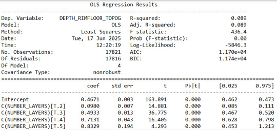
We can see a high F number and a very low p, so we can assume that at least two layer groups have different mean depths.

sub3 = sub1[['NUMBER_LAYERS', 'DEPTH_RIMFLOOR_TOPOG']].dropna() print ('means for depth by layer number') m2= sub3.groupby('NUMBER_LAYERS').mean() print (m2) print ('standard deviations for depth by layer number') sd2 = sub3.groupby('NUMBER_LAYERS').std() print (sd2)

It seems like deeper craters are most likely to have more layers but are there layers that cannot be differentiated based on its depth?

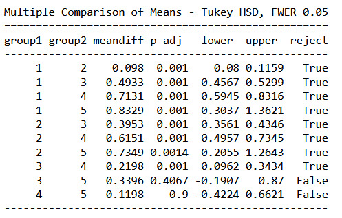
mc1 = multi.MultiComparison(sub1['DEPTH_RIMFLOOR_TOPOG'], sub1['NUMBER_LAYERS']) res1 = mc1.tukeyhsd() print(res1.summary())

The Turkey post hoc comparisons show that indeed craters with 1 to 4 layers have different mean depths.

5-layered craters have different mean depths in comparison with 1- and 2-layered craters only. So there is no significant difference between 5-layered crater and craters with 3 or 4 layers.

Layers vs Diameter

We can repeat this using the crater diameter as our response variable.

# using ols function for calculating the F-statistic and associated p value model2 = smf.ols(formula='DIAM_CIRCLE_IMAGE ~ C(NUMBER_LAYERS)', data=sub1) results2 = model2.fit() print (results2.summary())

Repeating this with the crater diameter shows that the wider craters are most likely to have more layers as well.

mc2 = multi.MultiComparison(sub1['DIAM_CIRCLE_IMAGE'], sub1['NUMBER_LAYERS']) res2 = mc2.tukeyhsd() print(res1.summary())

Here we see a similar pattern than with the crater depth. 5 Layer craters have similar mean depths that 3 and 4 layered ones, so it cannot be said that 5 layered craters are necessarily wider than 3 or 4 layered craters, but certainly wider than 1 or 2 layered ones.

[pabloatech]

Beerdays in a year depending on divorce of parents and moderated by sex

I run an anova for the quantitative variable "days a year beer is consumed" related to the categorical variable "parents divorced before respondant was 18 years old". There was no significant relevance for the categorical explanation. However, by introducing a moderator as the respondent sex (male/female), the categorical variable became relevant for the female respondents (p-value 0.0259<0.05).

Here you can see the python code:

import numpy import pandas import statsmodels.formula.api as smf

import statsmodels.stats.multicomp as multi

data = pandas.read_csv('C:/Users/zop2si/Documents/Statistic_tests/nesarc_pds.csv', low_memory=False)

convert data to numeric

data['S2AQ5B'] = pandas.to_numeric(data['S2AQ5B'], errors='coerce') # quantitative variable: how often drank beer in the last 12 months data['S1Q2D'] = pandas.to_numeric(data['S1Q2D'], errors='coerce') # categorical variable: parents got divorced before respondent was 18

subset adults age older than 18

sub1=data[data['AGE']>=18]

SETTING MISSING DATA

sub1['S2AQ5B']=sub1['S2AQ5B'].replace(99, numpy.nan) sub1['S1Q2D']=sub1['S1Q2D'].replace(9, numpy.nan)

recoding number of days when beer was drunk according to the nesarc documentation

recode1 = {1: 365, 2: 330, 3: 208, 4: 104, 5: 52, 6: 36, 7: 12, 8:11, 9: 6, 10: 2} sub1['BEERDAY']= sub1['S2AQ5B'].map(recode1)

converting new variable to numeric

sub1['BEERDAY']= pandas.to_numeric(sub1['BEERDAY'], errors='coerce')

ct1 = sub1.groupby('BEERDAY').size() print("Values in ct1 grouped by size of factor: ") print (ct1)

using ols function for calculating the F-statistic and associated p value

model1 = smf.ols(formula='BEERDAY ~ C(S1Q2D)', data=sub1) results1 = model1.fit() print (results1.summary())

drop empty rows from the model:

sub2 = sub1[['BEERDAY', 'S1Q2D']].dropna()

print(" ") print ('means for beerday by highest degree') m1= sub2.groupby('S1Q2D').mean() print (m1)

print(" ") print ('standard deviations for beerday by highest degree') sd1 = sub2.groupby('S1Q2D').std() print (sd1) print(" ") print(" ")

Check with the moderator parameter "sex"

sub11=data[(data['SEX']==1)] sub12=data[(data['SEX']==2)]

SETTING MISSING DATA

sub11['S2AQ5B']=sub11['S2AQ5B'].replace(99, numpy.nan) sub11['S1Q2D']=sub11['S1Q2D'].replace(9, numpy.nan) sub12['S2AQ5B']=sub12['S2AQ5B'].replace(99, numpy.nan) sub12['S1Q2D']=sub12['S1Q2D'].replace(9, numpy.nan)

recoding number of days when beer was drunk according to the nesarc documentation

recode1 = {1: 365, 2: 330, 3: 208, 4: 104, 5: 52, 6: 36, 7: 12, 8:11, 9: 6, 10: 2} sub11['BEERDAY']= sub11['S2AQ5B'].map(recode1) sub12['BEERDAY']= sub12['S2AQ5B'].map(recode1)

converting new variable to numeric

sub11['BEERDAY']= pandas.to_numeric(sub11['BEERDAY'], errors='coerce') sub12['BEERDAY']= pandas.to_numeric(sub12['BEERDAY'], errors='coerce')

print(" ") print ('association between BEERDAY, divorced parents before age of 18 and male sex') model2 = smf.ols(formula='BEERDAY ~ C(S1Q2D)', data=sub11).fit() print (model2.summary()) print(" ") print ('association between BEERDAY, divorced parents before age of 18 and female sex') model3 = smf.ols(formula='BEERDAY ~ C(S1Q2D)', data=sub12).fit() print (model3.summary())

create subsets for male and female to show the mean and std. deviation

m101 = sub11[['BEERDAY','S1Q2D']] m102 = sub12[['BEERDAY','S1Q2D']]

print(" ") print ("Means for BEERDAY for divorced parents (S1Q2D=1) or not (S1Q2D=1) for males") m3= m101.groupby('S1Q2D').mean() print (m3) print ("Std. dev. for BEERDAY for divorced parents (S1Q2D=1) or not (S1Q2D=1) for males") m31= m101.groupby('S1Q2D').std() print (m31) print(" ") print ("Means for BEERDAY for divorced parents (S1Q2D=1) or not (S1Q2D=1) for females") m4 = m102.groupby('S1Q2D').mean() print (m4) print ("Std. dev. for BEERDAY for divorced parents (S1Q2D=1) or not (S1Q2D=1) for females") m41 = m102.groupby('S1Q2D').std() print (m41)

Results:

OLS Regression Results

Dep. Variable: BEERDAY R-squared: 0.000 Model: OLS Adj. R-squared: 0.000 Method: Least Squares F-statistic: 1.739 Date: Wed, 14 May 2025 Prob (F-statistic): 0.187 Time: 07:23:34 Log-Likelihood: -97052. No. Observations: 16123 AIC: 1.941e+05 Df Residuals: 16121 BIC: 1.941e+05 Df Model: 1

Covariance Type: nonrobust

coef std err t P>|t| [0.025 0.975]

Intercept 74.6835 1.708 43.727 0.000 71.336 78.031

C(S1Q2D)[T.2.0] -2.5351 1.922 -1.319 0.187 -6.303 1.233

Omnibus: 5083.122 Durbin-Watson: 2.003 Prob(Omnibus): 0.000 Jarque-Bera (JB): 12184.626 Skew: 1.809 Prob(JB): 0.00 Kurtosis: 5.247 Cond. No. 4.15

association between BEERDAY, divorced parents before age of 18 and male sex

OLS Regression Results

Dep. Variable: BEERDAY R-squared: 0.000 Model: OLS Adj. R-squared: 0.000 Method: Least Squares F-statistic: 1.902 Date: Wed, 14 May 2025 Prob (F-statistic): 0.168 Time: 07:23:35 Log-Likelihood: -60187. No. Observations: 9856 AIC: 1.204e+05 Df Residuals: 9854 BIC: 1.204e+05 Df Model: 1

Covariance Type: nonrobust

coef std err t P>|t| [0.025 0.975]

Intercept 92.3883 2.450 37.706 0.000 87.585 97.191

C(S1Q2D)[T.2.0] -3.7765 2.738 -1.379 0.168 -9.144 1.591

Omnibus: 2149.253 Durbin-Watson: 2.001 Prob(Omnibus): 0.000 Jarque-Bera (JB): 3831.912 Skew: 1.458 Prob(JB): 0.00 Kurtosis: 3.909 Cond. No. 4.27

association between BEERDAY, divorced parents before age of 18 and female sex

OLS Regression Results

Dep. Variable: BEERDAY R-squared: 0.001 Model: OLS Adj. R-squared: 0.001 Method: Least Squares F-statistic: 4.963 Date: Wed, 14 May 2025 Prob (F-statistic): 0.0259 Time: 07:23:35 Log-Likelihood: -36051. No. Observations: 6267 AIC: 7.211e+04 Df Residuals: 6265 BIC: 7.212e+04 Df Model: 1

Covariance Type: nonrobust

coef std err t P>|t| [0.025 0.975]

Intercept 50.3890 2.015 25.012 0.000 46.440 54.338

C(S1Q2D)[T.2.0] -5.1098 2.294 -2.228 0.026 -9.606 -0.614

Omnibus: 3438.368 Durbin-Watson: 2.014 Prob(Omnibus): 0.000 Jarque-Bera (JB): 20897.128 Skew: 2.688 Prob(JB): 0.00 Kurtosis: 10.151 Cond. No. 3.97

Mean and std. dev.:

Means for BEERDAY for divorced parents (S1Q2D=1) or not (S1Q2D=1) for males BEERDAY S1Q2D 1.0 92.388295 2.0 88.611836 Std. dev. for BEERDAY for divorced parents (S1Q2D=1) or not (S1Q2D=1) for males BEERDAY S1Q2D 1.0 110.622748 2.0 108.107760

Means for BEERDAY for divorced parents (S1Q2D=1) or not (S1Q2D=1) for females BEERDAY S1Q2D 1.0 50.388966 2.0 45.279214 Std. dev. for BEERDAY for divorced parents (S1Q2D=1) or not (S1Q2D=1) for females BEERDAY S1Q2D 1.0 79.780063 2.0 75.152691

[my100sul]

[ryhanpz]

Analysis of Variance (ANOVA) in Political Systems and Life Expectancy

This blog explores the application of Analysis of Variance (ANOVA) to examine how life expectancy varies across different political systems. The analysis utilizes a dataset from the Gapminder Project, which includes country-level indicators of health, wealth, and development for a specific year.

The Dataset: Gapminder

The dataset used in this analysis is sourced from the Gapminder Project, containing various indicators of health, wealth, and development for multiple countries. For this specific analysis, two main variables are of interest:

Life Expectancy: A quantitative variable representing the average life expectancy in different countries.

Polity Category: A categorical variable that classifies countries based on their polity score. This score indicates the level of democracy in a country and is divided into three categories:

Autocracy (polity score ≤ -1)

Anocracy (0 ≤ polity score ≤ 5)

Democracy (polity score ≥ 6)

The Code: ANOVA Implementation

import numpy import pandas import statsmodels.formula.api as smf import statsmodels.stats.multicomp as multi

# Reading a subset of data to avoid memory issues

data = pandas.read_csv('gapminder.csv', low_memory=False)

# Converting polityscore to numeric

data['polityscore'] = pandas.to_numeric(data['polityscore'], errors='coerce') data['lifeexpectancy'] = pandas.to_numeric(data['lifeexpectancy'], errors='coerce')

# Categorizing democracy score values

def categorize_polity(score): if pandas.isna(score): return 'Unknown' elif score <= -1: return 'Autocracy' elif 0 <= score <= 5: return 'Anocracy' elif score >= 6: return 'Democracy' else: return 'Unknown'

data['polity_category'] = data['polityscore'].apply(categorize_polity)

# Subsetting data: keep only rows with valid lifeexpectancy and polity category

sub1 = data[['lifeexpectancy', 'polity_category']].dropna() sub1 = sub1[sub1['polity_category'] != 'Unknown']

# Checking the number of entries in each category

ct1 = sub1.groupby('polity_category').size() print(ct1)

# ANOVA analysis: is life expectancy different based on democracy category?

model1 = smf.ols(formula='lifeexpectancy ~ C(polity_category)', data=sub1) results1 = model1.fit() print(results1.summary())

# Mean and standard deviation for each category

print('Means for lifeexpectancy by polity category:') m1 = sub1.groupby('polity_category').mean() print(m1)

print('Standard deviations for lifeexpectancy by polity category:') sd1 = sub1.groupby('polity_category').std() print(sd1)

# Post hoc test: Tukey HSD

mc1 = multi.MultiComparison(sub1['lifeexpectancy'], sub1['polity_category']) res1 = mc1.tukeyhsd() print(res1.summary())

================================================

ANOVA Model Interpretation:

When examining the association between life expectancy (quantitative response) and polity category (categorical explanatory), an Analysis of Variance (ANOVA) revealed significant differences in life expectancy across the different polity categories (Autocracy, Anocracy, and Democracy). The results showed that individuals living in Democratic countries had a significantly higher life expectancy (Mean = 71.82, s.d. ±9.45) compared to those in Anocratic (Mean = 62.06, s.d. ±8.64) and Autocratic countries (Mean = 65.83, s.d. ±9.52). The F-statistic was 13.41 (with degrees of freedom 2, 157) and the p-value was 4.18e-06 (0.00000418), indicating strong statistical significance.

This suggests that life expectancy varies significantly based on the political system in place. Note that the degrees of freedom for the F-statistic (2, 157) are derived from the OLS table as the DF model (2) and DF residuals (157). In this case, the F-statistic value of 13.41 comes from the OLS table, and the very small p-value (4.18e-06) confirms that the differences in life expectancy across the polity categories are statistically significant.

Post Hoc Test Interpretation:

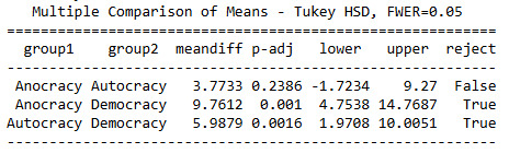
To further explore where the significant differences lie, post hoc comparisons using the Tukey HSD test were performed. The results from the post hoc test revealed that life expectancy in Democratic countries was significantly higher compared to Anocratic countries (Mean difference = 9.76, p = 0.001) and Autocratic countries (Mean difference = 5.99, p = 0.0016). However, the difference between Autocratic and Anocratic countries (Mean difference = 3.77, p = 0.2386) was not statistically significant, meaning there was no substantial difference in life expectancy between these two groups.

The Tukey HSD test shows that those in Democratic countries enjoy significantly better life expectancy outcomes than those in more autocratic or mixed political systems.

[krcmarik]

ANOVA work

The work below is based on the 'Outlook on Life' dataset. The primary question that I looked at was how different groups perceive the treatment of the criminal justice system based on race.

I looked at two explanatory variables, first gender and second race. The response variable was a numerical rating from 1 to 7, with 1 being equal treatment and 7 being unequal treatment. The question asked by the researchers was whether or not minorities receive equal treatment as whites in the criminal justice system.

Looking at gender first, I rejected the 'null' hypothesis since the p-value was less than 0.05 (6.65e-6). Average ratings from women (2) were higher than men (1), meaning that women perceive less equality in the criminal justice system than men do. When I looked at just the averages (5.07 vs 5.46), I thought that this would not be a significant difference. But statistically it is. This is why it's important to 'check the math' and not just go on your gut feeling.

Looking at race second, I rejected the 'null' hypothesis since the p-value was less than 0.05 (1.48e-158). The Tukey post hoc test showed that group 2 (black) were different than the four comparison groups and had the highest rating (6.18). Group 1 (white) had the lowest rating (3.87) was different than three of the other groups - the only group that they were similar to was group 5 (2+ races), which had an average rating of 3.96. These results mean that whites have the highest perception of equal treatment of minorities in the criminal justice system and blacks have the lowest.

code{

import numpy import pandas import statsmodels.formula.api as smf import statsmodels.stats.multicomp as multi

data = pandas.read_csv('ool_pds.csv', low_memory=False)

setting variables you will be working with to numeric

data['W1_K4'] = pandas.to_numeric(data['W1_K4'])

subset data to those who answered according to the rating system (1-7), excluding refused (-1) and not sure (9)

sub1=data[(data['W1_K4']>=1) & (data['W1_K4']<=7)] #& (data['PPETHM']>=3) & (data['PPETHM']<=4)]

ct1 = sub1.groupby('W1_K4').size() print (ct1)

using ols function for calculating the F-statistic and associated p value

model1 = smf.ols(formula='W1_K4 ~ C(PPGENDER)', data=sub1) results1 = model1.fit() print (results1.summary())

sub2 = sub1[['W1_K4', 'PPGENDER']].dropna()

print ('means for rating of criminal justice treatment by gender') m1= sub2.groupby('PPGENDER').mean() print (m1)

print ('standard deviations for rating of criminal justice treatment by gender') sd1 = sub2.groupby('PPGENDER').std() print (sd1)

by race

sub3 = sub1[['W1_K4', 'PPETHM']].dropna()

model2 = smf.ols(formula='W1_K4 ~ C(PPETHM)', data=sub3).fit() print (model2.summary())

print ('means for rating of criminal justice treatment by race') m2= sub3.groupby('PPETHM').mean() print (m2)

print ('standard deviations for rating of criminal justice treatment by race') sd2 = sub3.groupby('PPETHM').std() print (sd2)

mc1 = multi.MultiComparison(sub3['W1_K4'], sub3['PPETHM']) res1 = mc1.tukeyhsd() print(res1.summary())

}

results {

W1_K4 1 170 2 112 3 91 4 165 5 343 6 317 7 800 dtype: int64

OLS Regression Results

Dep. Variable: W1_K4 R-squared: 0.010 Model: OLS Adj. R-squared: 0.010 Method: Least Squares F-statistic: 20.40 Date: Mon, 21 Apr 2025 Prob (F-statistic): 6.65e-06 Time: 14:03:17 Log-Likelihood: -4162.2 No. Observations: 1998 AIC: 8328. Df Residuals: 1996 BIC: 8340. Df Model: 1

Covariance Type: nonrobust

coef std err t P>|t| [0.025 0.975]

Intercept 5.0651 0.064 79.114 0.000 4.940 5.191

C(PPGENDER)[T.2] 0.3940 0.087 4.517 0.000 0.223 0.565

Omnibus: 234.131 Durbin-Watson: 1.893 Prob(Omnibus): 0.000 Jarque-Bera (JB): 319.632 Skew: -0.973 Prob(JB): 3.91e-70

Kurtosis: 2.777 Cond. No. 2.72

Notes: [1] Standard Errors assume that the covariance matrix of the errors is correctly specified. means for rating of criminal justice treatment by gender W1_K4 PPGENDER 1 5.065076 2 5.459108 standard deviations for rating of criminal justice treatment by gender W1_K4 PPGENDER 1 1.989139 2 1.904511

OLS Regression Results

Dep. Variable: W1_K4 R-squared: 0.310 Model: OLS Adj. R-squared: 0.308 Method: Least Squares F-statistic: 223.4 Date: Mon, 21 Apr 2025 Prob (F-statistic): 1.48e-158 Time: 14:03:17 Log-Likelihood: -3802.3 No. Observations: 1998 AIC: 7615. Df Residuals: 1993 BIC: 7643. Df Model: 4

Covariance Type: nonrobust

coef std err t P>|t| [0.025 0.975]

Intercept 3.8666 0.062 62.148 0.000 3.745 3.989 C(PPETHM)[T.2] 2.3130 0.078 29.469 0.000 2.159 2.467 C(PPETHM)[T.3] 0.9027 0.268 3.374 0.001 0.378 1.427 C(PPETHM)[T.4] 1.1855 0.177 6.693 0.000 0.838 1.533

C(PPETHM)[T.5] 0.0977 0.313 0.312 0.755 -0.517 0.712

Omnibus: 153.821 Durbin-Watson: 1.924 Prob(Omnibus): 0.000 Jarque-Bera (JB): 189.998 Skew: -0.715 Prob(JB): 5.53e-42

Kurtosis: 3.488 Cond. No. 10.3

Notes: [1] Standard Errors assume that the covariance matrix of the errors is correctly specified. means for rating of criminal justice treatment by race W1_K4 PPETHM 1 3.866569 2 6.179532 3 4.769231 4 5.052083 5 3.964286 standard deviations for rating of criminal justice treatment by race W1_K4 PPETHM 1 2.006179 2 1.306314 3 1.769055 4 1.755411 5 2.301081

Multiple Comparison of Means - Tukey HSD, FWER=0.05

group1 group2 meandiff p-adj lower upper reject

1 2 2.313 0.001 2.0987 2.5273 True 1 3 0.9027 0.0068 0.1723 1.633 True 1 4 1.1855 0.001 0.7019 1.6691 True 1 5 0.0977 0.9 -0.7577 0.9531 False 2 3 -1.4103 0.001 -2.1326 -0.688 True 2 4 -1.1274 0.001 -1.5987 -0.6562 True 2 5 -2.2152 0.001 -3.0637 -1.3668 True 3 4 0.2829 0.885 -0.5595 1.1252 False 3 5 -0.8049 0.2663 -1.9038 0.2939 False

4 5 -1.0878 0.0159 -2.0406 -0.135 True

}

[yappacadaver]

goddddd i miss model 1 so badddddddddddd i can't even lie T_T

[maria-mga2024mi5017]

11 second club animation - Fixing the issue with the 'Chubby' rig

16/03/2025

Hi everyone. So, I'm having a few issues with the 'chubby rig' and I'm planning to fix them now.

The main issue being the fact that the eyes pop out every time I try to animate the head. If this continues to happen, I won't be able to animate the character's expressions at all...

Advice from Krishantha -

During one of Krishantha's sessions, I was able to get his contact in case of any issues when doing class activities. Luckily, I was able to get some advice from him today to sort out this issue with the 'Chubby' rig.

Basically, what he mentioned was that I will have to save the rigs in a separate folder and then into the animation file. I will be mentioning the steps to this down below.

Step 1 (Saving your downloaded rigs): -

Go to advance skeleton > select your demo rigs (both the male and female rig) > save them in the 'rigs' folder (go to destop > create a rigs folder > create two separate folders inside called 'male_rig' and 'female_rig' and then save the rigs in the relevant folders as MAYA BINARY files.

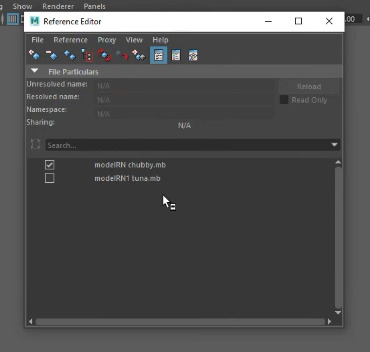
Step 2 (referencing rigs to the animation scene): -

Open new scene > file > reference editor > click on the 1st plus icon > select the rig (you will have to repeat this step for the 2nd rig) > reference

When using this picker, make sure to select between model and model1 when animation the characters!

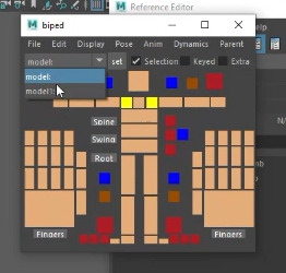
If you want to hide any of your rigs, untick them from the box next to their names. The model will still be there in the scene!

Step 3 (Saving the animation file with the 2 rigs): -

File > save scene as > desktop > Rigs folder > create a folder called animation > inside the 'animation folder', save this file as '01_blocking' (or anything else) as a MAYA ASCII file

Step 4 (Import your environment into the animation folder):-

File > Import > select your environment > Place it in the scene

Step 5 (Copying animation from your old/issue file and saving it to you referenced rig file): -

Now this step isn't necessary to follow unless you have an issue during the animating process. (Which was my main issue)

Even though there are issues in my old file, I can copy and paste the animation work I've done there into the new file (In the animation folder)

Go to the animation picker > click all (Advanced skeleton with basically copy all the animation in the controllers) > Anim tab > copy

2. Then go to your new file > go to the animation picker/biped > select the right model > select all > anim tab > paste

In conclusion, you should always reference your rigs. That way, you will hardly come across any issues with the rig mesh! (Like the eyes popping out in my case)

[marulaakapane]

so i got a mapel! actually an upgrade from my prev one (model1), but the speech synth sounds exactly like pam!!!! <3

[jagdelf]

[DIECASTTEAM] 1/64 レクサス LFA

気になっていたDIECASTTEAMのLFAを店頭で発見！棚にはオレンジ、ガンメタ、そしてアイスブルー…散々悩んだ結果、実車に存在しなさそうなこれを選んでみた。定番色は別のメーカーからも出そうだし、白のシートがカッコよかったのです。

先行していたMODEL1版と比べると、スタイリングと仕上げで勝り、各部のメッシュやマフラー、内装なんかの作り込みは一歩譲る印象。どちらか選ぶのなら個人的にはコッチかなあ。サスペンションギミック付きなのはちょっと意外で面白い。<874>