#WavePropagation

[renovatio06]

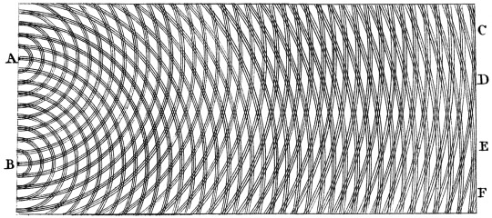
The surprising origins of wave-particle duality

Everything acts like a wave while it propagates, but behaves like a particle whenever it interacts. The origins of this duality go way back. Credit: Thomas Young & Sakurambo/Wikimedia Commons Source: The surprising origins of wave-particle duality Who would’ve thought? I hadn’t been aware that the discovery of the wave-particle duality of photons, electrons and even larger structures of particles…

[kozmolog]

🌌 Evrenin İçi Boş Mu?: Eter Teorileri Uzay deyince akla yıldızlar, meteorlar, gezegenler, süper novalar ya da karadelikler geliyor. Bugüne kadar uzay denilince akla gelen şeyler sınırlıdır. Oysa akla gelmeyen bir şey daha var. Link bio'da. https://kozmolog.net/2021/09/16/evrenin-ici-bos-mu-eter-teorileri/ Yazan: Murat Tetik #timedilation #michelsonmorley #einstein #electromagnetic #wavepropagation #nasa #rocketscience #astrophysics #theoreticalphysics #generalrelativity #lorentz #michelsonmorleyexperiment #eterteorisi #ethertheory #tesla #relativitytheory #relativity relativitytheory #relativity #questioneverything #physics #physicslecture #physicslectures #interferometry #interferometer #sciencelectures https://www.instagram.com/p/CT4zgjLIXbJ/?utm_medium=tumblr

[your-article-is-too-long]

How Does Fire Spread?

This is supplementary material for my Triplebyte blog post, “How Does Fire Spread?”

The following code creates a cellular automaton forest fire model in Python. I added so many comments to this code that the blog post became MASSIVE and the code block looked ridiculous, so I had to trim it down.

… but what if someone NEEDS it?

# The NumPy library is used to generate random numbers in the model. import numpy as np # The Matplotlib library is used to visualize the forest fire animation. import matplotlib.pyplot as plt from matplotlib import animation from matplotlib import colors # A given cell has 8 neighbors: 1 above, 1 below, 1 to the left, 1 to the right, # and 4 diagonally. The 8 sets of parentheses correspond to the locations of the 8 # neighboring cells. neighborhood = ((-1,-1), (-1,0), (-1,1), (0,-1), (0, 1), (1,-1), (1,0), (1,1)) # Assigns value 0 to EMPTY, 1 to TREE, and 2 to FIRE. Each cell in the grid is # assigned one of these values. EMPTY, TREE, FIRE = 0, 1, 2 # colors_list contains colors used in the visualization: brown for EMPTY, # dark green for TREE, and orange for FIRE. Note that the list must be 1 larger # than the number of different values in the array. Also note that the 4th entry # (‘orange’) dictates the color of the fire. colors_list = [(0.2,0,0), (0,0.5,0), (1,0,0), 'orange'] cmap = colors.ListedColormap(colors_list) # The bounds list must also be one larger than the number of different values in # the grid array. bounds = [0,1,2,3] # Maps the colors in colors_list to bins defined by bounds; data within a bin # is mapped to the color with the same index. norm = colors.BoundaryNorm(bounds, cmap.N) # The function firerules iterates the forest fire model according to the 4 model # rules outlined in the text. def firerules(X): # X1 is the future state of the forest; ny and nx (defined as 100 later in the # code) represeent the number of cells in the x and y directions, so X1 is an # array of 0s with 100 rows and 100 columns). # RULE 1 OF THE MODEL is handled by setting X1 to 0 initially and having no # rules that update FIRE cells. X1 = np.zeros((ny, nx)) # For all indices on the grid excluding the border region (which is always empty). # Note that Python is 0-indexed. for ix in range(1,nx-1): for iy in range(1,ny-1): # THIS CORRESPONDS TO RULE 4 OF THE MODEL. If the current value at # the index is 0 (EMPTY), roll the dice (np.random.random()); if the # output float value <= p (the probability of a tree being growing), # the future value at the index becomes 1 (i.e., the cell transitions # from EMPTY to TREE). if X[iy,ix] == EMPTY and np.random.random() <= p: X1[iy,ix] = TREE # THIS CORRESPONDS TO RULE 2 OF THE MODEL. # If any of the 8 neighbors of a cell are burning (FIRE), the cell # (currently TREE) becomes FIRE. if X[iy,ix] == TREE: X1[iy,ix] = TREE # To examine neighbors for fire, assign dx and dy to the # indices that make up the coordinates in neighborhood. E.g., for # the 2nd coordinate in neighborhood (-1, 0), dx is -1 and dy is 0. for dx,dy in neighborhood: if X[iy+dy,ix+dx] == FIRE: X1[iy,ix] = FIRE break # THIS CORRESPONDS TO RULE 3 OF THE MODEL. # If no neighbors are burning, roll the dice (np.random.random()); # if the output float is <= f (the probability of a lightning # strike), the cell becomes FIRE. else: if np.random.random() <= f: X1[iy,ix] = FIRE return X1 # The initial fraction of the forest occupied by trees. forest_fraction = 0.2 # p is the probability of a tree growing in an empty cell; f is the probability of # a lightning strike. p, f = 0.05, 0.001 # Forest size (number of cells in x and y directions). nx, ny = 100, 100 # Initialize the forest grid. X can be thought of as the current state. Make X an # array of 0s. X = np.zeros((ny, nx)) # X[1:ny-1, 1:nx-1] grabs the subset of X from indices 1-99 EXCLUDING 99. Since 0 is # the index, this excludes 2 rows and 2 columns (the border). # np.random.randint(0, 2, size=(ny-2, nx-2)) randomly assigns all non-border cells # 0 or 1 (2, the upper limit, is excluded). Since the border (2 rows and 2 columns) # is excluded, size=(ny-2, nx-2). X[1:ny-1, 1:nx-1] = np.random.randint(0, 2, size=(ny-2, nx-2)) # This ensures that the number of 1s in the array is below the threshold established # by forest_fraction. Note that random.random normally returns floats between # 0 and 1, but this was initialized with integers in the previous line of code. X[1:ny-1, 1:nx-1] = np.random.random(size=(ny-2, nx-2)) < forest_fraction # Adjusts the size of the figure. fig = plt.figure(figsize=(25/3, 6.25)) # Creates 1x1 grid subplot. ax = fig.add_subplot(111) # Turns off the x and y axis. ax.set_axis_off() # The matplotlib function imshow() creates an image from a 2D numpy array with 1 # square for each array element. X is the data of the image; cmap is a colormap; # norm maps the data to colormap colors. im = ax.imshow(X, cmap=cmap, norm=norm) #, interpolation='nearest') # The animate function is called to produce a frame for each generation. def animate(i): im.set_data(animate.X) animate.X = firerules(animate.X) # Binds the grid to the identifier X in the animate function's namespace. animate.X = X # Interval between frames (ms). interval = 100 # animation.FuncAnimation makes an animation by repeatedly calling a function func; # fig is the figure object used to resize, etc.; animate is the callable function # called at each frame; interval is the delay between frames (in ms). anim = animation.FuncAnimation(fig, animate, interval=interval) # Display the animated figure plt.show()

[nocklebeast]

caustics and catastrophes where the Elwha River meets the Salish Sea 25 July 2019. Lower Elwha River. Port Angeles, WA.   #elwha #salishsea #caustics #catastrophes #wavepropagation #optics #leicasl #wave #waves #interference #24-90VarioElmarit (at Lower Elwha, Washington) https://www.instagram.com/p/B0eK8AcnIB9/?igshid=1sfk4odamrdtz

[rickdrako]

View this post on Instagram

A post shared by Ricardo Mondragon (@rickdrako)

Optical Interference #sound #sine #waves #channel #rgb #waves #wavepropagation #study #chichao #art #artist #visuals (at North Center, Chicago)

[a-bette-day-group]

Select your interactions. Program by Behrouz. #Physicsphilosophylove #physics #philosophy #love #interference #waves #wavepropagation #bb (at Santa Monica, California)

[dioni-macaroni]

Soul Propagation

People ask what I look for in individuals or what I would want in a relationship and the closest I can get to describing my desire is as one for constructive interference.