#Worksheet_Change

[kareamemad]

اسهل واسرع كود فى منع الادخالات المكررة فى الاكسل Remove Duplicated Value In Excel

اسهل واسرع كود فى منع الادخالات المكررة فى الاكسل Remove Duplicated Value In Excel   بسم الله الرحمن الرحيم اهلا بكم متابعى موقع عالم الاوفيس كود جديد من مكتبة اكواد الاكسل vba اسهل واسرع كود فى منع الادخالات المكررة فى الاكسل Remove Duplicated Value منع الإدخالات المكررة في جدول Excel له أهمية كبيرة للعديد من الأسباب. إليك بعض الأسباب الرئيسية لمنع الإدخالات المكررة: 1. الدقة والموثوقية: من خلال منع الإدخالات المكررة، يمكنك ضمان الدقة والموثوقية في بياناتك. إذا كانت هناك إدخالات مكررة في جدول Excel، فقد يؤدي ذلك إلى الخلط والتباس ويمكن أن يؤثر على نتائج التحليل أو العمليات الأخرى التي تعتمد على هذه البيانات. 2. توفير المساحة: بمنع الإدخالات المكررة، يمكنك توفير مساحة في جدول Excel. إدخال البيانات المكررة يؤدي إلى زيادة حجم الملف واستهلاك موارد النظام، وبالتالي يمكن أن يؤثر على أداء الجدول. 3. تسهيل التحليل والفرز: عندما يكون لديك بيانات نظيفة وخالية من الإدخالات المكررة، يمكنك تسهيل عمليات التحليل والفرز. يمكنك استخدام الوظائف والتصفيات في Excel بشكل فعال للتعامل مع البيانات الفريدة والمميزة. 4. تجنب الأخطاء والتكرار: من خلال منع الإدخالات المكررة، يمكنك تجنب الأخطاء والتكرار في البيانات. إدخال نفس القيمة مرارًا وتكرارًا قد يؤدي إلى النسيان أو الإغفال، ويمكن أن يتسبب في إعاقة سير العمل والإنتاجية. الكود المستخدم فى الشرح Private Sub Worksheet_Change(ByVal Target As Range) If Application.WorksheetFunction.CountIf(Range("a:a"), Target) > 1 Then MsgBox "Duplicted Value", vbCritical Target.Value = "" End If End Sub لحماية البيانات ومنع الإدخالات المكررة في جدول Excel، يمكنك استخدام أدوات مثل التحقق من الصحة (Data Validation) وإزالة النسخ المكررة (Remove Duplicates) والتنسيقات المشروطة (Conditional Formatting) وغيرها من الميزات المتاحة في برنامج Excel. قد يعجبك ايضا  تحميل برنامج حركة الخزينة مجانا اسطوانة التعريفات الشاملة DriverPack Solution بدون نت  شيت بجميع اكواد الخدمة في فورى Fawry اكواد فوري برنامج مجانى لمتابعة حركة الخزينة Excel تحميل برنامج مخازن مجانى 100 % كامل ومفتوح المصدر | Store Management System  برنامج متابعة الشيكات (شيكات دفع / شيكات قبض ) Cheques Management + نسخة تجريبية   تحميل برنامج الكاشير2020 المجانى لادارة حسابات المحلات التجارية Cashier  تحميل برنامج مجانى حضور وانصراف الموظفين بالبصمة( دوام الموظفين المجانى)  تحميل برنامج مخازن مجانى 100% -برنامج المنجز 2024 تحميل برنامج محاسبى كامل كفعل مدى الحياة تحميل برنامج الايرادات والمصروفات مجانى 100% تحميل برنامج تنظيم الملفات والسكرتارية وادارة مكاتب المحاماة اسهل طريقة لعمل دواير حمراء بناء على محتوى الخلية (تحديد الناجح من الراسب ) تحميل يوزرفورم كامل للبحث متعدد المعايير تحميل Free Office 2024  مجانا تحميل قاعدة بيانات الطلاب اكسس مفتوحة المصدر مجانا تحميل برنامج ادارة العيادات الطبية اكسس مجانا مفتوح المصدر تحميل مجانى برنامج المخازن والمبيعات (عملاء – موردين –فواتير – مصروفات – تفدقات تقدية ) بالاكسيس مفتوح المصدر تحميل جدول دوام الموظفيين جاهز بالاكسل  تحميل اوفيس 365 تحميل مجانى برنامج ادارة وتتبع العقود والوثائق الرسمية قوالب وملفات اكسل مجانا     اكسل متقدم via عالم الاوفيس https://ift.tt/Pd1EhqX May 05, 2024 at 03:03PM

[kotaexcel]

イベント処理でシートの変化を他のシートに反映させる

今回はイベント処理を使います。

まずはコードから。

Private Sub Worksheet_Change(ByVal Target As Range)    If Not Intersect(Target, Range("C1")) Is Nothing Then        Sheets("sample").Range("C1") = Range("C1")    End If End Sub

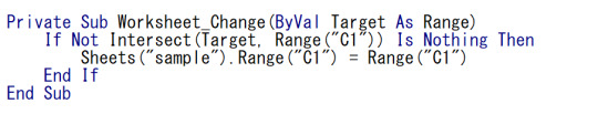
これを対象のワークシートモジュールに記述します。

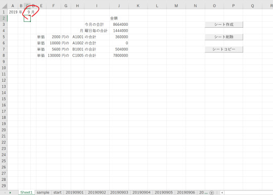
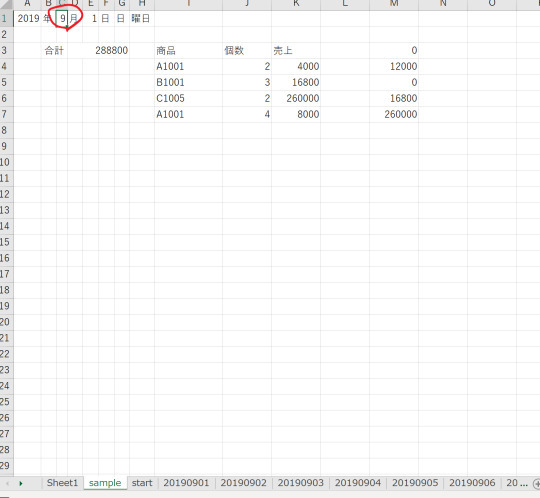
今回は売上表の日付を変更すると、sample（シートコピーのもとになるシート）の日付が変更されるようになっています。

このように、こちらからマクロを実行しなくても、条件に合わせて実行するプロシージャをイベントプロシージャといいます。

イベントプロシージャは、マクロ名が決まっています。

今回の場合は、セルの内容が変化したらマクロが起動される「Worksheet_Change」です。

Targetには変更されたセルが格納されています。

ですので、目的のセルが変更したかどうかを確認するために、Intersectを使っています。これは共通部分があるときに、その共通するセルを返すものです。

ですので、これがNothingでない……つまり空でないときにマクロの中身が実行されるようにすればいいわけですね。

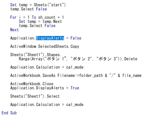
ちなみに、このようにシートにマクロを保存したので、これをコピーして保存しよとすると、「マクロ対応の形式で保存してください」と言われてしまいます。

ですので、シートをコピーするマクロでは、早めにDisplayAlertsをFalseにするようにして、ファイル形式がマクロなしのまま保存されるようにしました。

[exceltricks]

So können Sie mehrere Einträge aus einer Liste (Datenüberprüfungsliste, Gültigkeitsliste) auswählen

Wenn Sie in einer Zelle eine Liste über die Datenüberprüfung (Gültigkeitsregel) in Excel hinterlegen, dann können Sie standardmäßig immer nur einen Listeneintrag auswählen.

Die Excel-Expertin Mynda Treacy hat auf YouTube hierzu ein interessantes Video veröffentlicht (Quelle: https://youtu.be/l8a6EvihDpc). Durch den Einsatz eines ereignisgesteuerten Makros (Worhsheet_Change) ist es möglich, dass…

[exceldepo]

Mükerrer Tarih Kontrolü Yapma, yazılan tarihlerin daha önce yazılıp yazılmadığının kontrol edilmesini sağlayan kodlar içermektedir. Excel'de mükerrer kayıtları kontrol etme oldukça önemli hususların başında gelmektedir. Bu mükerrer kontrole, farklı alanlarda ihtiyaç duyulmaktadır. Bizde bu içeriğimizde, yazılan iki tarih arasındaki değerlerin daha önce yazılıp yazılmadığının kontrol edilmesini ele aldık. Yapılan kontrol, başlangıç ve bitiş tarihlerini içeren iki tarihe ait mükerrer girişlerin engellenmesine yöneliktir. En çok, izin takip sistemlerini Excel ile yapanlarda ihtiyaç duyulmaktadır. Dosyadaki kodlar, sayfanın Worksheet_Change olayına yazılmıştır. Yani, belirtilen iki sütunda tarih yazılmışsa devreye girmektedir. Hemen akabinde ise, yeni yazılan iki tarihin daha önce yazılıp yazılmadığı kontrol edilmektedir. Dosyada, iki tarihe ilave olarak kontrolün ikinci aşamasında çalışan bazlı olması sağlanmaktadır. Yani, tarihler sadece çalışanlara göre kontrol edilmektedir. Eğer farklı bir çalışana ait iki tarih girilirse, sorunsuz bir şekilde yazılması sağlanmaktadır. Mükerrer Tarih Kontrolü Yapma Sonuç Dosyamız, iş hayatının hemen her aşamasında kullanılacak nitelikte faydalı bir örnektir. Bu tür ihtiyacı olan ya da makro kodlarına meraklı kullanıcılarımıza fayda sağlaması temennisiyle. [button color="black" size="medium" link="https://www.exceldepo.com/dosyalar/mukerrer-tarih-kontrolu-yapma.12449/" icon="fa-download" target="true" nofollow="false" sponsored="true"]Excel İndir[/button]

[felchevansblog]

Excel Tutorials - Worksheet VBA Events

Introduction to Worksheet VBA Events

In this tutorial, we will introduce you to worksheet VBA events. You will learn how to write code that runs in response to various Event Planning Companies that occur in a workbook or worksheet.

We will start by discussing the three main types of events: workbook events, worksheet events, and chart events. We will then show you how to write code that runs in response to each type of event.

Workbook Events

Workbook events occur when a workbook is opened or closed, or when certain actions are taken on a workbook (such as saving or printing). You can write code that runs in response to these events.

For example, you could write code that automatically saves a backup copy of a workbook every time it is saved. Or, you could write code that checks for errors before a workbook is closed.

Worksheet Events

Worksheet events occur when a worksheet is activated or deactivated, or when certain actions are taken on a worksheet (such as adding or deleting data). You can write code that runs in response to these events.

For example, you could write code that automatically updates charts whenever data on the worksheet changes. Or, you could write code that checks for errors before data is entered into a worksheet.

How to Use Worksheet VBA Events

If you want to know how to use VBA events in your worksheets, this tutorial is for you. We'll cover everything you need to know, from what events are available to how to write code that will run when those events occur.

Events are a crucial part of programming in VBA. They allow you to write code that will execute in response to specific actions taken by the user or by the Excel application itself. In this tutorial, we'll focus on worksheet-level events. That is, events that are triggered by actions taken on a worksheet, such as opening or closing it, entering or changing data, and so on.

There are a few things to keep in mind when working with events:

1. Events happen as a result of some action taken by the user or Excel. For example, if you enter a value into a cell, that triggers the Worksheet_Change event. If you save a workbook, that triggers the Workbook_BeforeSave event.

2. You can't predict exactly when an event will occur - they happen asynchronously, which means your code needs to be prepared to handle them at any time.

3. When an event occurs, Excel calls your code automatically - you don't need to do anything special to make it happen. Just make sure your code is written and saved in the right place (more on that later).

4. Many events have an "Application

Different Types of Worksheet VBA Events

There are several different types of VBA events that can occur while a worksheet is open. Each type of event has its own associated code that will execute when the event occurs. The most common types of events are:

-Activate: This event occurs when a worksheet is activated. Use this event to initialize values or perform other actions when a worksheet is first opened.

-Deactivate: This event occurs when a worksheet is deactivated. Use this event to save values or perform other actions when a worksheet is closed.

-Calculate: This event occurs whenever a cell on the worksheet is calculated. Use this event to track changes to cell values or to perform complex calculations.

-Change: This event occurs whenever a cell on the worksheet is changed. Use this event to track changes to cell values or to perform other actions based on user input.

Pros and Cons of Using Worksheet VBA Events

When it comes to automating your Excel workbook, you have a few different options available to you. One option is to use worksheet VBA events. This can be a great way to automate certain tasks in your workbook, but there are also some potential drawbacks that you should be aware of.

One advantage of using worksheet VBA events is that they can be triggered automatically based on certain conditions. For example, you could set up an event to run a macro whenever a cell in a particular range is changed. This can be a great time-saver if you have a lot of data that needs to be processed regularly.

Another advantage of worksheet VBA events is that they can help you keep track of changes made to your workbook. Every time an event is triggered, it is logged in the Event Log sheet. This can be helpful for troubleshooting purposes or for auditing purposes.

There are also some potential disadvantages to using worksheet VBA Event Management Services . One disadvantage is that they can slow down your workbook if there are too many events being triggered at once. Another disadvantage is that they can be tricky to debug if something goes wrong. If you're not careful, it's easy to accidentally write code that will cause an infinite loop of events being triggered.

Overall, worksheet VBA events can be a great way to automate tasks in your workbook. Just be aware of the potential drawbacks and make sure you test your code

Conclusion

Overall, Excel VBA events are a powerful way to automate various actions in your worksheets. By understanding how they work and how to use them, you can save yourself a lot of time and effort. In this tutorial, we've covered the basics of VBA events and how to use them in your own worksheets. Experiment with different events and see what you can come up with!

[hiyoko-channnel]

こんなExcelは嫌だ！【イベントマクロの紹介】

麗かな音楽にのせて、イベントマクロのご紹介～！ 初めてこれを知った時は感動しました。 0:00　Worksheet_SelectionChange イベント 1:57　Worksheet_Change イベント 3:57　WorkBook_Open イベント 5:58　WorkBook_NewSheet イベント ＜Twitter＞ わちょん ＜チャンネル紹介＞ ExcelやVBA中心。時には真剣に、時には楽しく【ゆっくり動画】を作っています ＜動画編集ソフト＞ ゆっくりMovieMaker4 ＜音楽・効果音＞ 甘茶の音楽工房 さん 効果音ラボ…

[greysgiga]

Compare two columns in excel and return differences

#Compare two columns in excel and return differences update

#Compare two columns in excel and return differences code

#Compare two columns in excel and return differences update

I am in the middle of taking it out and prepping it for deployment as it was bought as a spare, and a switch is failing calling for it to be replaced. I have configured it but I want to update the firmware. I have a HP Procurve 2920 Switch (Bought 2010). Will my HP Procurve Take Aruba firmware? Hardware.It is provided as an example and a starting point for your development.

#Compare two columns in excel and return differences code

This is Air Code - I have neither compiled nor tested it. Private Sub Worksheet_SelectionChange(ByVal Target As Range) Why did I write this as a separate procedure (rather than, for example, the Worksheet_Change event procedure on the worksheet)? Well, we want to call this procedure whenever something changes on either worksheet so we can share this procedure by coding each worksheet's Worksheet_Change event procedure like this: You can use the Worksheet.Change event to call this procedure. So, when should this procedure be called? I would suggest calling it every time any value on either of the two worksheets changes. ' the colors in case the row was marked asįirstSheet.Range(Cells(index1, 1), Cells(index1, 4)).Interior.Color = vbWhiteįirstSheet.Range(Cells(index1, 1), Cells(index1, 4)).Font.Color = vbBlackįirstSheet.Range(Cells(index1, 1), Cells(index1, 4)).Interior.Color = vbYellowįirstSheet.Range(Cells(index1, 1), Cells(index1, 4)).Font.Color = vbRed ' the two sheets change, so we need to RESET ' to be called repeatedly as the values on ' (We do this because we expect this procedure ' If we DIDN'T find a match, we want to mark ' We've found a row on the second sheet that & secondSheet.Cells(index2, SECONDCOLUMN2) SecondValue = secondSheet.Cells(index2, FIRSTCOLUMN2) _ ' Loop through the rows on the second sheet ' Keep track of whether we've found a match & firstSheet.Cells(index1, SECONDCOLUMN1) ' For each row, concatenate the values from the two cellsįirstValue = firstSheet.Cells(index1, FIRSTCOLUMN1) _ ' Loop through the rows on the first worksheet Set secondSheet = ActiveWorkbook.Sheets(secondSheetName) Set firstSheet = ActiveWorkbook.Sheets(firstSheetName) Public Sub CompareSheets(firstSheetName As String, secondSheetName As String) The procedure looks like this:Ĭonst FIRSTCOLUMN1 As Integer = 2 'Column BĬonst SECONDCOLUMN1 As Integer = 3 'Column CĬonst FIRSTCOLUMN2 As Integer = 1 'Column AĬonst SECONDCOLUMN2 As Integer = 3 'Column C Whenever a row on the first sheet fails to have a match somewhere on the second sheet, this procedure will change the colors of the row to make its error status visible. I've put together some code that will perform this process. The procedure (I prefer not to use the term "macro" because in Excel that can, and should, refer to an MS Excel 4.0 Macro, which is a completely different and much uglier beast) will need to have two nested loops: an outer loop to scan the rows on the first sheet, and an inner loop to scan the rows on the second sheet. You have correctly concluded that you will need to use VBA to fulfill your requirements. However, let's ignore that and try to come up with an answer to your question. As John has pointed out, this thread is in the wrong forum - it should be in the Visual Basic for Applications (VBA) forum ( http:/ / / groups/ technical-functional/ vb-vba-l) rather than the SQL Server forum ( http:/ / / groups/ technical-functional/ sql-server-l).

[hyla12345]

Private Sub Worksheet_Change(ByVal Target As Range) Dim wCellVal As String

   'セルの値を取得する    With Worksheets("Sheet1")        wCellVal = .Cells(Target.Row, Target.Column).Value    End With

   'A列(ID)の文字数チェックを行う    If Target.Column = 1 Then        If Len(wCellVal) > 10 Then            MsgBox "IDは10桁以内で入力してください。", vbOKOnly + vbExclamation, "入力エラー"            Exit Sub        End If    End If

   'A列(ID)の半角チェックを行う    If Target.Column = 1 Then        If Len(wCellVal) <> LenB(StrConv(wCellVal, vbFromUnicode)) Then            MsgBox "IDは半角で入力してください。", vbOKOnly + vbExclamation, "入力エラー"            Exit Sub        End If    End If

   'B列(商品名)の全角チェックを行う    If Target.Column = 2 Then        If Len(wCellVal) * 2 <> LenB(StrConv(wCellVal, vbFromUnicode)) Then            MsgBox "商品名は全角で入力してください。", vbOKOnly + vbExclamation, "入力エラー"            Exit Sub        End If    End If

   'C列(品番)の半角チェックを行う    If Target.Column = 3 Then        If Len(wCellVal) <> LenB(StrConv(wCellVal, vbFromUnicode)) Then            MsgBox "品番は半角で入力してください。", vbOKOnly + vbExclamation, "入力エラー"            Exit Sub        End If    End If

   'D列(単価)の数字チェックを行う    If Target.Column = 4 Then        If Not IsNumeric(wCellVal) Then            MsgBox "単価は数字で入力してください。", vbOKOnly + vbExclamation, "入力エラー"            Exit Sub        End If    End If

End Sub

[officecommoffice-blog]

How To Use Nested If Statements In Microsoft office Excel And An Alternative VBA Solution

A common task in Excel is to define category names based on values; for example, grouping test scores into grades. A standard formula in Excel can do the job for a simple if then else scenario, but for multiple selections, the syntax can become complicated.

Let’s look at a simple set of test scores and the formula in the adjacent cell to define the result as passed or not achieved. 45 =if(a1>=50,”Passed”,”Not achieved”)

Excel And Nested If Formulas The problem occurs when we need to assess values based on multiple ranges. In our example, if we wanted to assess a score of between 50 and 65 as “average” the following formula applies: =if(and(a1>=50,a1

But this formula doesn’t allow for scores outside the “average” range such as the criteria for assessing scores below: Below 50 = “Not achieved” 50-65= “Average” Over 65=”Above average” The formula for applying the above conditions is complex: =IF(A1=50,A165,”Above average”)))

Clearly, the nested formula can become cumbersome and difficult to debug so let’s look at an elegant VBA alternative. A VBA Solution For Assessing Multiple Ranges

There are several different methods for assessing multiple values in VBA, but the one we’ll use is the select case method.

One of the best things you can do when writing VBA code is to reflect on the code and consider how easy it is to follow. First, we’ll select a column to assess and to make the code easier to read, assign the grade column and the number of scores to their own variables.

Range(“a1”).CurrentRegion.Columns(1).Select gradeCol = Selection.Column + 1 items = Selection.Count Now, we’ll loop through the selection and assign a grade to each score. For x = 1 To items test = (x) ‘ we don’t really need to reset the grade variable but it’s good practice to do so. grade=””Select Case test Case 0 To 49 grade = “Not achieved”Case 50 to 65 grade = “Average”Case 66 To 100 grade = “Above average” End SelectCells(x, gradeCol).Value = grade

Next Points To Note Using a VBA solution rather than a direct Excel formula reduces the chance of error but a clear disadvantage is that the grade is not updated if the scores are adjusted in the future. One option to address this issue could be a VBA worksheet_change event so that whenever the scores were changed, the code would be repeated. A more challenging solution might be to develop code which would create the formula as text and insert it into the applicable cells.

Summary This scenario involved balancing the option of the correct solution – an Excel formula – with the use of easily written VBA code. It’s an example of where Excel users need to make decisions based on their knowledge level and the issue being addressed.

For more information click here : office.com/setup

Content Source :http://office-comoffice.com/blog/2019/04/20/how-to-use-nested-if-statements-in-microsoft-office-excel-and-an-alternative-vba-solution/

[googleexcel]

Track

Dim vOldVal 'Must be at top of module Private Sub Worksheet_Change(ByVal Target As Range) Dim bBold As Boolean If Target.Cells.Count > 1 Then Exit Sub On Error Resume Next With Application .ScreenUpdating = False .EnableEvents = False End With If IsEmpty(vOldVal) Then vOldVal = "Empty Cell" bBold = Target.HasFormula With Sheet2 .Unprotect Password:="Secret" If .Range("A1") = vbNullString Then .Range("A1:E1") = Array("CELL CHANGED", "OLD VALUE", _ "NEW VALUE", "TIME OF CHANGE", "DATE OF CHANGE") End If With .Cells(.Rows.Count, 1).End(xlUp)(2, 1) .Value = Target.Address .Offset(0, 1) = vOldVal With .Offset(0, 2) If bBold = True Then .ClearComments .AddComment.Text Text:= _ "OzGrid.com:" & Chr(10) & "" & Chr(10) & _ "Bold values are the results of formulas" End If .Value = Target .Font.Bold = bBold End With .Offset(0, 3) = Time .Offset(0, 4) = Date End With .Cells.Columns.AutoFit .Protect Password:="Secret" End With vOldVal = vbNullString With Application .ScreenUpdating = True .EnableEvents = True End With On Error GoTo 0 End Sub Private Sub Worksheet_SelectionChange(ByVal Target As Range) vOldVal = Target End Sub

[kareamemad]

دليلك الشامل فى فرز وترتيب البيانات فى الاكسل | Sort Data In Excel

دليلك الشامل فى فرز وترتيب البيانات فى الاكسل | Sort Data In Excel   بسم الله الرحمن الرحيم اهلا بكم متابعى موقع عالم الاوفيس دليلك الشامل فى فرز وترتيب البيانات فى الاكسل     فرز البيانات في الإكسل هو عملية مهمة تستخدم لتنظيم البيانات الموجودة في جداول البيانات. يُعد الإكسل واحدًا من أبرز الأدوات المستخدمة على مستوى العالم في مجال تحليل البيانات وإدارتها، ويتيح للمستخدمين العديد من الطرق لفرز البيانات بناءً على مجموعة معايير محددة. اليوم سوف نستعرض معكم طريقتان لفرز البيانات فى الاكسيل Sort Data عندما تكون لديك جدول بيانات في الإكسل وترغب في ترتيبه بطريقة محددة، يمكنك استخدام خاصية الفرز لتنفيذ ذلك بسهولة. يمكنك فرز البيانات بناءً على قيمة في عمود معين أو بناءً على مجموعة من الأعمدة المختلفة. الطريقة الاولى لترتيب البيانات في الإكسل، يمكنك اتباع الخطوات التالية:   1. حدد المجموعة التي تود فرزها. انتقِ الصفوف والأعمدة التي يجب أن تتضمن البيانات التي ترغب في ترتيبها. 2. من قائمة "بيانات" في شريط الأدوات، انقر على الزر "فرز". 3. ستظهر نافذة "الفرز والتصفية". تحت علامة التبويب "فرز"، حدد العمود الذي ترغب في ترتيب البيانات وحدد الترتيب الذي تفضله، ��ما في ذلك الترتيب التصاعدي (من الأقل إلى الأكبر) أو الترتيب التنازلي (من الأكبر إلى الأقل). 4. إذا كان لديك مجموعة معايير للفرز، انقر على زر "إضافة مستوى" وحدد العمود التالي الذي تود ترتيبه. يمكنك تكرار هذه الخطوة حسب الحاجة لإضافة مجموعة أخرى من معايير الفرز. 5. بمجرد اختيارك لجميع معايير الفرز المطلوبة، انقر على زر "موافق" لبدء ترتيب البيانات.   بعد تنفيذ هذه الخطوات، ستقوم الإكسل بفرز البيانات بناءً على المعايير التي حددتها. ستلاحظ أن الصفوف ستعرض الآن بترتيب مختلف بناءً على القواعد التي وضعتها. الطريقة الثانية  وهذة الطريقة التى تسهل علينا العمل وهى عن طريق كود سهل جدا وبسيط نقوم بادخالة فى حدث التغيير لورقة العمل تقوم بالضغط على ورقة العمل ثم كليك يمين View Code ونكتب الكود التالى Option Explicit   Private Sub Worksheet_Change(ByVal Target As Range) If Not Intersect(Target, Range("d:d")) Is Nothing Then         Range("a:d").Sort Key1:=Range("d1"), Order1:=xlDescending, Header:=xlYes     End If End Sub   End Sub   في الختام، يُعد فرز البيانات في الإكسل أداة قوية تمكّن المستخدمين من تنظيم البيانات وتحليلها بشكل أكثر فعالية. ستجد أن استخدام خاصية الفرز مفيد في إدارة البيانات الضخمة واستعراضها بطريقة منظمة وسهلة القراءة. لتحميل ملف العمل  اكسل متقدم via عالم الاوفيس https://ift.tt/LTfVmG0 June 16, 2023 at 07:43PM

[access-excel-tip]

New Post has been published on Access-Excel.Tips

New Post has been published on http://access-excel.tips/excel-dependent-dropdown-list/

Excel dependent dropdown list | dependent validation list

This Excel tutorial explains how to create dependent dropdown list where dropdown list values depend on another list value.

Excel dependent dropdown list / dependent validation list

Suppose you have a continent list in Excel (Asia, North America, South America, etc). When an user selects a continent from a dropdown list, the user can then select the second dropdown list which contains all the countries of your selected continent, so the country list is dependent on the continent value.

For example, if you Europe Country in A2, you can only select a list of Europe countries in B2.

  If you select Asia Country in A2, you can only select Asia countries in B2.

Setup Excel dependent drop down list

Step 1: Create a new worksheet and write down all the items your want to display in the validation lists

  Step 2: Name the data range of the first level data validation list (continent). Name it Continent_List for easy reference. We add underline in the Range Name because the Range Name does not allow space. To name the range, highlight A2:A4, and then type the name directly on the top left. Click here to learn how to create dynamic validation list.

  Next, name the data range of column B, C and D. The Range Name should be exactly same as the corresponding values in column A, replace any space with underline.

  Step 3: Create dropdown list for Continent

Setup a template in a new worksheet as below

  Select range A2:A8, then navigate to Data tab > Data Validation

  Enter information as below. The Source is the Name Range that we defined for continent.

  Step 4: Create dependent dropdown list

Select range B2:B8, then navigate to Data tab > Data Validation

  Setup the values as below.

To explain the formula in Source:

Substitute function is to replace space with underline. For example, if A2 value is Asia Country, Substitute converts the text into Asia_Country, it is because Name Range does not allow space

INDIRECT function is to convert the value in A2 into a Range Name. For example, if A2 value is Asia_Country, Indirect function converts this text into a Range, which contains values China, Hong Kong, Macau

Now the dependent dropdown list is ready for use.

Clear dependent validation list value if first level validation list is reselected

What happens if we select Spain in Country dropdown list, then we select Asia Country in Continent? Excel allows you to do that, but this is not right as Spain is a Europe Country.

  To prevent this error, we need to clear the Country whenever Continent is reselected with the help of Worksheet_Change Event.

Press ALT+F11 > select Sheet1 > copy and paste the below code

Private Sub Worksheet_Change(ByVal Target As Range)     If Not Intersect(Target, Range("A2:A8")) Is Nothing Then         Target.Offset(0, 1).ClearContents     End If End Sub

Now whenever you select a Continent, Country becomes blank.

[exceltricks]

Eine Zelle in Excel nach einer Eingabe automatisch sperren und vor weiteren Veränderungen schützen

Eine Zelle in Excel nach einer Eingabe automatisch sperren und vor weiteren Veränderungen schützen

In dem folgenden YouTube-Video bekommen Sie demonstriert, wie Sie eine Zelle nach einer Eingabe automatisch sperren und somit vor Veränderungen schützen können. Hierbei kommt ein ereignisgesteuerter Makro zum Einsatz, welcher automatisch gestartet wird, wenn ein bestimmtes Tabellenblatt (Worksheet) geändert wird (change). Der Makro wird durch das Ereignis Worksheet_Changeautomatisch…

Auf WordPress ansehen

[exceldepo]

Bağlantılı Açılan Listeler Oluşturma içeriğinde, scripting dictionary yöntemi ile iki açılan listenin uyumlu olarak kullanılması öğretilmektedir. Excel'de olası yazım yanlışlarının önüne geçmek için en iyi yöntem, Açılan Liste kullanmaktır. Bunu yapmak için, Excel'in Veri Doğrulama özelliğine manuel ya da dinamik veri aralıkları tanımlanmaktadır. Böylece, hücreye tıklandığında, sağ kısmında aşağı doğru bir ok belirir ve tıklandığında listeden verilerin gelmesi sağlanır. Doğrulama uygulanan hücrede başka bir şeyler yazmak mümkün değildir. Yani, sistem buna izin vermeyecektir. Dolayısıyla, yanlış bir yazımın hücreye eklenmesi böylece mümkün olmamaktadır. Açılan listeler, bizlerinde oldukça önem verdiği ve kullandığı faydalı bir Excel özelliğidir. Dosyamızda da, bu özellik için tamamen makrolar ile oluşturulan bir örnek yer almaktadır. İlk açılan listede, olmazsa olmaz şehir seçimi yapılmaktadır. Böylece, ülkemizin 81 ilinin isimleri ilk açılan listeye eklenmektedir. Bu listeleme işlemi, dosyanın açıldığı anda otomatik çalışan makrolar ile yapılmaktadır. Makronun işlevi, veriler sayfasında bulunan ve tekrar eden il isimlerini, scripting dictionary yöntemiyle bir kez listelemektir. Artık, il isimleri kolayca hücrede açılan listeye eklenmiştir. Listele eklenen bu veriler, dinamik olarak Veri Doğrulama'nın Liste özelliğine eklenmektedir. Yani, yeni bir il eklendiği anda Kaynak alanının referans aralığı genişlemektedir. İkinci aşamada, ikinci açılan listeye birinci açılan liste ile bağlantılı olan ilçe isimlerinin yazdırılmasına geçilmiştir. Buradaki işlemler, ilk aşamaya göre biraz daha dinamik niteliktedir. Çünkü, ilk listeden seçilen il ismine göre, ikinci listedeki ilçe isimlerinin değişmesi gerekmektedir. Burada da, yine makrolar ile veri tablosundaki ilçe isimleri sorgulanmış ve il ismiyle eşleşenler bir hücrede yazdırılmıştır. Yine aynı kodlarda, üst resimde görüldüğü gibi Kaynak alanının referans aralığı otomatik biçimde yazılmaktadır. Bu aralık, her seçilen il ismine göre farklılık göstermektedir. Bunu sağlayan ise Excel Makrolarıdır. Bağlantılı Açılan Listeler Oluşturma Sonuç Artık, son aşama olan verilerin seçilmesi kısmına geçelim. Bu aşamada, sayfanın Worksheet_Change koduna eklenen kodlar ile, listelerin seçilmesine bağlı işlemlerin yapılması sağlanmaktadır. Aslında, olayın en kritik noktası bu aşamadır. Çünkü, hem il seçimi hem de ilçe seçimini sağlayan makroların tetiklenmesi burada gerçekleşmektedir. Eğer Açılan Listelere ihtiyacınız varsa, bu örneğin kullanılması özellikle tavsiye edilmektedir. Ama, bir tık daha gelişmiş hali görmek istenirse, Şerit Menüde Açılan Listeler Oluşturma içeriği tercih edilmelidir. Dosyamızdan yararlanmanız temennisiyle. [button color="black" size="medium" link="https://www.exceldepo.com/dosyalar/birbiriyle-baglantili-acilan-listeler-olusturma.12075/" icon="fa-download" target="true" nofollow="false" sponsored="true"]Excel İndir[/button]

[exceltricks]

Ausführen eines Makros bei Änderung von bestimmten Zellen in Excel

Ausführen eines Makros bei Änderung von bestimmten Zellen in Excel

In der täglichen Excel-Praxis sollen Makros oft nur dann ausgeführt werden, wenn Werte in bestimmten Zellen erfasst oder geändert werden.  Dies können Sie erreichen, wenn Sie die Intersect-Methode auf ActiveCell und den Bereich anwenden, der die Schlüsselzellen enthält.

Wie Sie dies in Excel einstellen bzw. umsetzen können Sie unter dem folgenden Link nachlesen:

https://support.microsoft.com/de-d…

Auf WordPress ansehen

[exceltricks]

Ausführen eines Makros bei Änderung von bestimmten Zellen in Excel

Ausführen eines Makros bei Änderung von bestimmten Zellen in Excel

In der täglichen Excel-Praxis sollen Makros oft nur dann ausgeführt werden, wenn Werte in bestimmten Zellen erfasst oder geändert werden.  Dies können Sie erreichen, wenn Sie die Intersect-Methode auf ActiveCell und den Bereich anwenden, der die Schlüsselzellen enthält.

Wie Sie dies in Excel einstellen bzw. umsetzen können Sie unter dem folgenden Link nachlesen:

https://support.microsoft.com/de-d…

Auf WordPress ansehen