#decimation in time fourier transform

[andmaybegayer]

Last Monday of the Week 2023-04-24

oh my god it's full of stars

Listening: Recommendation off IRC, On Giacometti by Hania Rani, a Polish musician. Predominantly piano, some synth. Beautiful slow neo-classical. Here's Knots and Time.

Watching: Got back into Andor, I was watching it with my mother and we remembered that was a thing. Just hit the end of the heist. A weird way for a heist to go wrong! Very half-failure, most heist movies either do the perfect heist or have it all go to hell, this was an unusual middle ground.

Reading: Went on a Fast Fourier Transform kick as part of a larger project. Student papers are interesting because they're not usually groundbreaking or anything but because they're by, well, students, who are only just learning the thing as well, they tend to explain themselves more fully. This one comparing two implementations of a decimation in frequency DFT on FPGA's served as a useful jumping off point for a lot of other reading.

Playing: Not much, a little more screwing around in the Minecraft server I set up, I've established a pretty decent little base of operations and tamed some cats to keep Creepers away. I'm very heavily stealing my house design from Mine O' Clock which has the downside of really needing you to light up your surroundings, I've been ambushed by monsters while doing inventory management more than once.

Making: Finished sewing on patches for the penrose quilt, which is now officially officially done. I'll take pictures once they're cleaned, that quilt has been kicking around for a while and there's a lot of blood and spit and dirt in there.

Tools and Equipment: I picked up this little USB-C to barrel jack adapter for my laptop that seems to work, it just has a tiny trigger circuit to negotiate 20V power from the charger and passes it right on through.

My laptop can charge on USB-C but more than once when the power has cut something has tripped a protection circuit in the charging system so that it refuses to charge off USB-C for a while. It's first-generation PD hardware, known issues. As a result when I travel I've been carrying both my handy compact USB-C charger and the big stock charger so that if that happens I have a recovery method. Now that I have this, I can just carry this and use it for recovery instead.

You can get this class of item (barrel jack to USB-C adapter) pretty readily and it's a handy way to really pack down your laptop's support hardware if it's a little older and doesn't have USB-C charging, or if like mine its USB-C charging is a little unreliable. DeviantOllam did a little video on it a while ago but a) I cannot find it and b) it took a few years for the hardware to appear locally at affordable prices.

Dell and HP both have annoying DRM one-wire chips baked into their charging cables but neither of them will outright refuse to charge on raw 20V, they'll just complain and maybe slow your rate of charge a little.

[lifesciencepotluck]

Figuring out structure

Proteins are like molecular machines. Unlike actual machines, proteins can fold into intricate 3-D structures on their own. Wouldn't it be convenient if your bookshelf from IKEA could do that? If we want to understand how proteins work, we need a blueprint. Some parts of the protein are essential for stability; other parts are crucial for getting things done through binding or catalysis. We need to understand how different parts of the protein fit together; this is where Structural Biology comes in. Getting the 3-D structure is one of the main steps in characterising new anemone toxins. I will cover some of the techniques we use to investigate the toxin structure.

The hierarchy of protein structure goes like this: primary structure-->secondary structure-->tertiary structure-->quaternary structure. For anemone toxins, we don't have to worry about the quaternary structure. Usually, anemone toxins have one polypeptide, not multiple polypeptides.

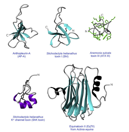
Figure 1. Structures of anemone toxins (Source: Norton, R. S, 2009)

Primary structure:

It's the amino acid sequence or 'code' for the protein. You can get the amino acid sequence from DNA, mRNA or protein sequencing. Protein sequencing just gives you the sequence for your protein. However, if we use DNA or mRNA sequencing, then we have to figure out the 'mature' peptide sequence. DNA and mRNA code for the 'first draft' of the peptide. After translating mRNA to protein, the signal peptide and pro-peptide are attached to the 'mature peptide.' Those two parts of the protein get cut out before our mature peptide can go out in the world and decimate prey.

Secondary structure:

Our flat polypeptide chain will fold into different secondary structures like alpha-helices, beta-sheets, beta turns, etc. Circular dichroism and Fourier transform infrared radiation (FT-IR) can tell us about the secondary structure of the toxin. CD and FT-IR are commonly used to predict the amount of each secondary structure in proteins. For CD, we measure how much of circularly polarised light in the far-UV region is absorbed by the sample. We use curve fitting programs to determine which combination of secondary structures fits the spectra the best (e.g. 50% beta-sheet, 10% alpha-helix, 20 % random coil and 20 % beta-turn). FT-IR works similarly, but we use infrared radiation instead of polarised light. FT-IR is a better option for investigating the interactions between pore-forming toxins and lipid membranes. The lipid vesicle or 'sacs' scatter polarised light, which it makes challenging to use CD for the same purpose.

One of the best things about spectroscopic techniques is that they are not as time-consuming as, X-ray crystallography. You can have multiple CD, and FT-IR runs in 1-2 hours and get the processed data before lunch. However, CD and FT-IR are low-resolution techniques. They don't tell you the exact position and orientation of tryptophan 32. We need atomic resolution structures to get an in-depth understanding of how anemone toxins work.

Tertiary structure:

The full 3-D structure of proteins will have secondary structure plus the disulphide linkages, salt bridges, hydrophobic interactions. There are two main ways of getting atomic resolution structures: X-ray crystallography and NMR. X-ray crystallography can give high-resolution 3-D structures—if you manage to please the crystal gods. If you don't have the ideal crystallisation conditions—no crystal for you. I know PhD students who spent 12-18 months on crystallising their protein. However, once you get past the crystallisation bottleneck, the diffraction experiments and data processing doesn't take as much time. In theory, you can get better resolution with X-ray crystallography than NMR. Let's assume you don't have time for crystallisation and you go with NMR. NMR is excellent for finding the structure of smaller proteins, but for larger proteins, you have to use isotopic labelling. Some proteins that are too big for NMR. In X-ray crystallography, the protein is a 'frozen' state. However, NMR also lets you study proteins in solution to understand the dynamics of the protein. You can observe how the protein changes when it binds to something.

We can also predict the 3-D structure of the toxin-based on the sequence alone.

How?

Computer magic !

With the protein data bank and structure prediction tools like SWISS-MODEL, you can predict the 3-D structure of a new toxin. If there is an anemone toxin in the database with an experimentally determined 3-D structure and it has high sequence similarity with your new toxin, you can use homolog modelling. If you can't use homology modelling, you can use de novo structure prediction like I-TASSER. In de novo modelling, the program predicts the structure for smaller sections of the protein and uses those bits to build the full predicted model. Model prediction isn't 100% accurate, and we still have to determine the 3-D structure experimentally. However, predicted 3-D structures act as a guide.

Every technique has its strengths and weaknesses. A good researcher tries to use the most suitable method for their project to its full potential. You have to realise the power that's inside.

So, what can you do once you have the 3-D structure of a toxin?

I am going to use APETx1 from the clonal anemone as an example. APETx1 is a potassium channel toxin, which targets the Ether-a-gogo channels in heart cells. Since APETx1 is a small potassium channel toxin, Chagot and company could use NMR. They found that APETx1 belong to the Defensin family. A variety of anti-bacterial proteins and ion channel toxins belong to this family. Proteins with Defensin-4 domain, have double or triple-stranded antiparallel b-sheets linked to a short a-helix by two disulphide bridges. Since NMR can reveal disulphide linkages, Chagot found APETx1 has an inhibitor cysteine knot (ICK). The inhibitor cysteine is a very popular protein fold because it's so stable that it makes proteins resilient against heat stress and proteolysis. Getting the structure of a toxin allows us to classify the toxin and compare it with structurally similar toxins. Since APETx1 has structurally similarity with two other toxins BeKm1 and CnErg1, you can infer it would have a similar mechanism for blocking potassium channels. Chagot suggested that five key amino acids on APETx1 (i.e. Tyr 5, Tyr 32, Phe33, Lys8 and Lys 18) 'block' the Ether-a-gogo channels through electrostatic interactions.

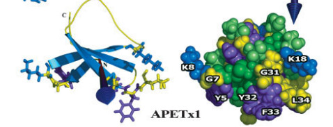
Figure 2. 3-D structure for APETx1 (Source: Chagot et al, 2005)

In short, we can use a variety of biophysical techniques to get structural information for new toxins  and the structure provides insight into the function. Protein structure and function are different sides of the same coin. Next time, I will flip the coin by covering how we figure out function.

Citations:

Chagot, B., Diochot, S., Pimentel, C., Lazdunski, M. & Darbon, H. Solution structure of APETx1 from the sea anemone Anthopleura elegantissima: A new fold for an HERG toxin. Proteins Struct. Funct. Genet. 59, 380–386 (2005).

Jouiaei, M. et al. Ancient venom systems: A review on cnidaria toxins. Toxins (Basel). 7, 2251–2271 (2015).

Norton, R. S. Structures of sea anemone toxins. Toxicon 54, 1075–1088 (2009).

Norton, R. S. & Pallaghy, P. K. The cystine knot structure of ion channel toxins and related polypeptides. Toxicon 36, 1573–1583 (1998).

Dauplais, M. et al. On the Convergent Evolution of Animal Toxins. J. Biol. Chem. 272, 4302–4309 (1997).

Belmonte, G. et al. Primary and secondary structure of a pore-forming toxin from the sea anemone, Actinia equina L., and its association with lipid vesicles. BBA - Biomembr. 1192, 197–204 (1994).

Honma, T. & Shiomi, K. Review Article Peptide Toxins in Sea Anemones: Structural and Functional Aspects. Mar. Biotechnol. 8, 1–10 (2006).

Bernard Gilquin, Judith Racape, Anja Wrisch, Violeta Visan, Alain Lecoq, Stephan Grissmer, Andre´Menez, and S. G. Structure of the BgK-Kv1.1 Complex based on distance restraints identified by double mutant cycles: Molecular basis for convergent evolution of Kv1 channel blockers. J. Biol. Chem. 277, 37406–37413 (2002).

[myprogrammingsolver]

Lab 7: Decimated-in-frequency FFT using the Butterfly Technique Solution

Lab 7: Decimated-in-frequency FFT using the Butterfly Technique Solution

Introduction FFT is a method of performing Discrete Fourier Transform which basically represents a time domain signal in terms of its components at different discretized frequency levels (fre-quency bins) . In this lab, we will design a Decimated-in -frequency (DIF) FFT Transform system for n=8 (See Fig.1). The twiddle factors are 9 bits wide and will be provided. Also, note that the…

[programmingsolver]

ECE Lab 7: Decimated-in-frequency FFT using the Butterfly Technique Solution

ECE Lab 7: Decimated-in-frequency FFT using the Butterfly Technique Solution

Introduction FFT is a method of performing Discrete Fourier Transform which basically represents a time domain signal in terms of its components at different discretized frequency levels (fre-quency bins) . In this lab, we will design a Decimated-in -frequency (DIF) FFT Transform system for n=8 (See Fig.1). The twiddle factors are 9 bits wide and will be provided. Also, note that the…

[fastcompression]

Fast Discrete Wavelet Transform on CUDA

Wavelet analysis, which is the successor of the Fourier analysis, is based on the idea that the same information, the same signal can be represented in different forms, depending on the purpose. To translate a signal into another form, a basis is first chosen - a set of linearly independent functions, and the signal is represented as a sum of these functions with some coefficients. In the Fourier analysis, the basis consists of periodic harmonic functions sin(k*x) and cos(k*x), corresponding to oscillations with a certain frequency throughout the domain of definition. Thus, having obtained the Fourier transform of a signal, we can determine its frequency spectrum and see which oscillations it consists of. If the signal characteristics change (for example, in time for sound signals or in space for images), then we can decompose it into components by using wavelet analysis, in which the basis consists of shifts and scales of a certain mother wavelet function. In such representation of a signal, we can track changes in the frequency spectrum, as well as study the local structure of the signal at a certain frequency, at a certain scale.

The representation of data in the form of wavelet coefficients is usually more compact than the original representation. From the perspective of the information theory, such a representation has less entropy. Moreover, such a representation also allows to obtain an approximation of the original signal with a given accuracy, by using only a fraction of the wavelet coefficients. Due to this, 2D Discrete Wavelet Transform is actively used in image compression (e.g. in popular formats JPEG2000 and DJVU). And due to the ability of transition to multi-scale representation of data, it is also used in image enhancement algorithms, such as noise reduction, filtering, fast scaling, and in artificial intelligence applications, such as feature extraction and segmentation, in compressed sensing applications during signal reconstruction.

The Discrete Wavelet Transform (DWT) of a signal is obtained by sequential applying of two filters (low-pass and high-pass) with decimation to eliminate redundancy. Such an algorithm is called the Mallat algorithm and can be used both for decomposition and for reconstruction. As a result, a signal is decomposed into two components: approximation (lower resolution version) and details. By applying this decomposition repeatedly to low-frequency coefficients, a multi-scale decomposition is obtained, which is called dyadic. This allows us to obtain (and to adjust) information on a wider frequency spectrum: at each decomposition step, the frequency spectrum is doubled, and the minimum resolution is halved.

Since images are two-dimensional, their DWT-transformation is performed both vertically and horizontally. The result is four fragments (subbands) with half the width and half the height, one of which is a smaller copy of the image (LL subband), and the three remaining subbands contain information about the details – horizontal (HL), vertical (LH) and diagonal (HH). At each subsequent step of decomposition, the LL subband is replaced by four smaller subbands, so the total number of subbands increases by three. Similarly, an algorithm is constructed for signals of a higher dimension (e.g. for video sequences as 3D signals or for time-varying computed tomography results as 4D signals).

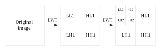
Fig. 1. Subbands of 2D wavelet coefficients after the first and the second DWT of an image

Many applications of the DWT are time-critical. Therefore, computation of the transform is often boosted by using specialized processors or accelerators, such as FPGA, accelerators with Intel MIC architecture, GPU graphics processors. GPUs have an excellent price-performance ratio and performance to power consumption ratio. Moreover, high-level programming platforms OpenCL and NVIDIA CUDA have contributed to their widespread use in various calculations due to the smooth learning curve, detailed documentation, and an extensive set of examples.

How to implement fast parallel DWT processing?

As a rule, instead of the Mallat separable convolutional algorithm, a lifting scheme is used for computation of DWT, because it has a number of theoretical and practical advantages. Among the theoretical advantages: it is easier to understand and explain (it is not relied on the Fourier transform), and the inverse transform is easily obtained by performing lifting steps in the reverse order. Moreover, if we use integer arithmetic, the absence of loss of accuracy (perfect reversibility) is guaranteed. Practical advantages are a smaller number of arithmetic operations (up to a factor of two), the ability to transform signals of arbitrary length (not only a multiple of 2n), possibility of fully in-place calculation (no auxiliary memory is needed). In addition, the lifting scheme can be used to construct wavelets of the second generation, in which the basis does not necessarily consist of shifts and scales of a certain function.

A considerable amount of research was performed on implementation of the wavelet transform on various platforms, including modern GPUs. The first studies were devoted to the comparison of the separable convolution-based algorithm and the lifting scheme, then the attention of researchers was completely switched to the effective implementation of the lifting scheme. The main difficulty that must be overcome when implementing a lifting scheme on GPU is the need of data exchange between threads after each lifting step. On GPU, data exchange within the threads of a single thread block is performed via shared memory, the size of which is very limited, while data exchange between thread blocks is relatively slow due to global memory access and synchronization of all threads of the kernel. Therefore, in order to achieve the best performance, it is necessary to choose such size of thread blocks and such size of arrays in shared memory that would balance the time for threads synchronization and the time for redundant calculations that are inevitable when the source data is divided into blocks.

For parallel processing of a two-dimensional image on the GPU, different strategies were proposed that can be divided into three groups:

Row-Column (RC)

Block-Based (BB)

Sliding window (SW)

RC methods transform an image as a whole, and a transposition operation is often used to speed up the vertical transformation. When the original image is too large, implementations from the first group will suffer from a lack of shared memory. Moreover, the performance of this approach is limited due to the need to write intermediate results (after column transformation) to global memory.

BB methods transform an image by dividing it into smaller blocks, and the row-column method is applied to each of them separately. Note that the correct result is achieved only in the case when these blocks overlap, where the blocks are extended in each direction on a few pixels depending on the type of wavelet. Such implementations use a limited amount of shared memory, independent of the image size, and they access global memory less frequently compared to RC methods.

Finally, methods of the third group transform an image by using column slabs with sliding window within each slab. The window allows you to keep intermediate results in shared memory longer. As a result, such methods can be considered a hybrid of the first two approaches.

After optimizations and implementations of all three methods, the researchers showed that the BB method is the most efficient, so we've chosen it for our implementation. Within this approach, the original image is divided into blocks of width M and height N, which need to be expanded by four pixels (four for a 4-step lifting scheme of CDF 9/7 and two for a 2-step lifting scheme of CDF 5/3) in each direction. As a result, intersecting blocks of size (M + 8) × (N + 8) can be processed without separate conditions for the boundary pixels. Parameters M and N are chosen empirically to maximize the performance.

Wavelets CDF 9/7 and CDF 5/3

The Cohen-Daubechies-Feauveau (CDF) wavelets belong to the family of biorthogonal wavelets, which, unlike orthogonal wavelets, can be symmetric. They were made popular by Ingrid Daubechies, and two members of this wavelet family (CDF 9/7 and CDF 5/3) are now used in the JPEG2000 image compression. The CDF 9/7 wavelet has four vanishing moments, which means that the corresponding high-frequency wavelet coefficients of a cubic polynomial signal are zero. The CDF 5/3 wavelet has only two vanishing moments, but its main feature is the existence of an integer implementation, which has no loss of accuracy (arising with most of the other wavelets due to rounding of irrational numbers). Due to this property of CDF 5/3, JPEG2000 algorithm has lossless compression mode.

Hardware and software for DWT benchmarking

CPU Intel Core i7-5930K (Haswell-E, 6 cores, 3.5–3.7 GHz)

GPU NVIDIA GeForce GTX 1080 (Pascal, 20 SMM, 2560 cores, 1.6–1.7 GHz)

OS Windows 10 (x64), version 1803

CUDA Toolkit 10.0

Fastvideo Image & Video Processing SDK 0.14.1

GPU DWT benchmarks

We've measured the DWT performance for CDF 9/7 and CDF 5/3 wavelets on 24-bit images (8 bits in each of 3 color channels) of different sizes (up to 8K Ultra HD). The number of DWT levels ranged from 1 to 5. The obtained results include only the processing time on GPU, because it is assumed that the original data is already in the GPU memory, and the result of the transformation will be written to the same memory.

From the tables and the figures you can see, that the two-level DWT is ~40% slower than the single-level DWT, while the five-level DWT is ~60% slower. It could be also seen, that the performance of DWT saturates on large images when there is enough work to load each multiprocessor of GPU.

Optimized DWT implementations of CDF 5/3 and CDF 9/7 are utilized in our JPEG2000 codec on CUDA.

Table 1. GPU DWT performance for 4K image (3840×2160, 24-bit)

Wavelet | DWT levels | Time, ms | Performance, GB/s | Frames per second

CDF 5/3 (int) | 1 | 1.28 | 18.2 | 784

CDF 5/3 (int) | 2 | 1.78 | 13.0 | 563

CDF 5/3 (int) | 5 | 2.10 | 11.8 | 476

CDF 9/7 (float) | 1 | 1.29 | 18.0 | 777

CDF 9/7 (float | )2 | 1.78 | 13.0 | 563

CDF 9/7 (float) | 5 | 2.10 | 11.8 | 476

Table 2. GPU DWT performance for 8K image (7680×4320, 24-bit)

Wavelet | DWT levels | Time, ms | Performance, GB/s | Frames per second

CDF 5/3 (int) | 1 | 4.28 | 21.6 | 233

CDF 5/3 (int) | 2 | 6.03 | 15.4 | 166

CDF 5/3 (int) | 5 | 6.79 | 13.7 | 147

CDF 9/7 (float) | 1 | 4.28 | 21.6 | 233

CDF 9/7 (float) | 2 | 6.18 | 15.0 | 162

CDF 9/7 (float) | 5 | 6.86 | 13.5 | 146

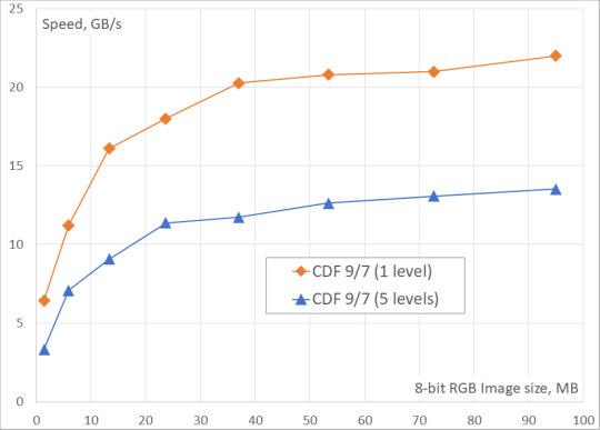
Fig. 2. Fastvideo DWT performance benchmarks on GeForce GTX 1080 for images of different sizes

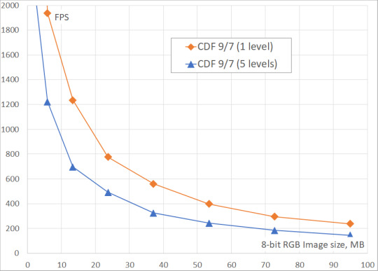
Fig. 3. Fastvideo DWT frame rate on GeForce GTX 1080 for images of different sizes

Original article see at: https://www.fastcompression.com/benchmarks/benchmarks-dwt.htm

[joshuallee86]

An Introduction to the Fast Fourier Transform

This article will review the basics of the decimation-in-time FFT algorithms.

[algorithms-en-blog]

Butterfly diagram

This article is about butterfly diagrams in FFT algorithms; for the sunspot diagrams of the same name, see Solar cycle. Signal-flow graph connecting the inputs x (left) to the outputs y that depend on them (right) for a "butterfly" step of a radix-2 Cooley–Tukey FFT. This diagram resembles a butterfly (as in the Morpho butterfly shown for comparison), hence the name, although in some countries it is also called the hourglass diagram. In the context of fast Fourier transform algorithms, a butterfly is a portion of the computation that combines the results of smaller discrete Fourier transforms (DFTs) into a larger DFT, or vice versa (breaking a larger DFT up into subtransforms). The name "butterfly" comes from the shape of the data-flow diagram in the radix-2 case, as described below. The earliest occurrence in print of the term is thought to be in a 1969 MIT technical report. The same structure can also be found in the Viterbi algorithm, used for finding the most likely sequence of hidden states. Most commonly, the term "butterfly" appears in the context of the Cooley–Tukey FFT algorithm, which recursively breaks down a DFT of composite size n = rm into r smaller transforms of size m where r is the "radix" of the transform. These smaller DFTs are then combined via size-r butterflies, which themselves are DFTs of size r (performed m times on corresponding outputs of the sub-transforms) pre-multiplied by roots of unity (known as twiddle factors). (This is the "decimation in time" case; one can also perform the steps in reverse, known as "decimation in frequency", where the butterflies come first and are post-multiplied by twiddle factors. See also the Cooley–Tukey FFT article.) More details Android, Windows

[electronicstuff96-blog]

DSP Programming in Matlab

DSP Programming in Matlab

As in our last post we had discussed about Digital signal processor, In this post we will try to compute the DFT, FFT and convolution of a input signal  on a  Matlab.

What is DFT ?

DFT is said to be a frequency domain representation of the original input sequence.In DFT input signal is periodic and the output we get after DFT computation is also periodic.The discrete Fourier transform (DFT)…

[electronicstuff96-blog]

Digital signal processing

click below for pdf

Dsp assignment solution pdf

visit tomorrow for remaining.

Thank you..!!!