#fixing my vlookup formulas

[copperbadge]

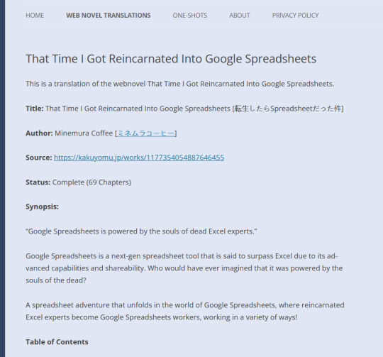
Me: Okay, but I....I would read this.

Also Me: ...you know you can, the URL is right in the screencap.

This Novel: Is actually pretty fun even in a poor machine translation.

"Oops, I forgot to explain. This is Google Spreadsheets, and we are its workers."

Oh no, I don't understand why, I feel like dying. What does it mean to be in Google Spreadsheets, not in heaven or another world?

[ID: A screengrab of a web novel archival site, kakuyomu.jp, featuring a story translated into English from Japanese. The title is "That Time I Got Reincarnated Into Google Spreadsheets" by author Minemura Coffee, complete in 69 chapters (nice). The synopsis begins, "Google Spreadsheets is powered by the souls of dead Excel experts."]

Well that's a webnovel title that I've yet to see til now

[patrice-bergerons]

hi Alex!! i hope you don't mind, but if i have an excel question 👉👈 basically i have a long long list of items, each with its price. i want to make smaller lists of different combinations of items, and have it auto-populate a column with the prices for each list. if i have the full list of each item with its price, is there a way to get my smaller lists to auto-populate with the price from this?? hope this makes sense and sorry for the random ask 😭😭

Please it makes my day every time I get an excel question 🥰🥰🥰

It sounds like what you need is the =VLOOKUP() function which can "look up" prices from the long list to populate the shorter list. Here is a mock up:

I have a fake long list in cells A1 thru A5 and a fake short list in A9:10. To find the price for mangoes I entered the vlookup formula into cell B9. It takes 4 values (separated by commas in the above- if you are using excel in a different language the separator might be something else)

What do you need to be looked up? Here the answer is a mango, which is entered into cell A9, so I said A9. The $ in front of the A tells Excel to fix the column reference. In other words even if you copy the same formula to cell C9, it would still reference column A, not B (which is what it would have done sans fixing)

Where do you want this to be looked up? The answer is the long list so I gave the full range for it. The $A$1 notation fixes the entire range, so regardless of what column or row you copy your formula into it will keep referencing the same range.

Which column's values do you want me to return? Here price is in the second column of the referenced array so we say 2. If your second column contained e.g. colour and prices were in the 3rd, we would have made our reference range $A$1:$C$6 above and said 3 here.

Do you want me to look things up based on the vibes? 😎 NEVER trust excel to vibe so we say false, i.e. give me an exact match. Idk what's up with the mobile app but in my computer I don't enter the () after false.

You can then hit copy with the cell selected and paste the formula into the rest of your small list and voila, prices!

Vlookup can look up values across different tabs and it can be made more dynamic than the simple example I have above. There are also other more complicated formulas that are even more dynamic. Conversely all this formula business can be quite confusing when you are new to it. My DMs are fully open if you have questions, follow-ups, or the above does not work for you!

For further reference here is the formula for grape:

On my computer, when I had just written the formula in B9 and hit enter, I would have selected B9 and B10 and then hit Ctrl + D which would drag the formula down to B10. As an alternative to copying cell B9 and pasting it onto B10.

[zachrantekulturu2013-blog1]

9 SMARTER Tips on how to USE EXCEL FOR ENGINEERING

As an engineer, you’re almost certainly making use of Excel virtually every day. It doesn’t matter what industry you're in; Excel is made use of Everywhere in engineering. Excel may be a immense plan using a great deal of awesome likely, but how can you know if you’re working with it to its fullest abilities? These 9 recommendations will help you begin to obtain essentially the most out of Excel for engineering. one. Convert Units devoid of External Tools If you’re like me, you most likely do the job with numerous units regular. It is 1 on the wonderful annoyances within the engineering lifestyle. But, it’s turned out to be much much less annoying due to a function in Excel which will do the grunt work to suit your needs: CONVERT. It’s syntax is: Would like to understand much more about sophisticated Excel techniques? View my absolutely free training just for engineers. In the three-part video series I'll show you ways to fix complex engineering difficulties in Excel. Click right here to obtain began. CONVERT(variety, from_unit, to_unit) Wherever quantity stands out as the value which you desire to convert, from_unit is definitely the unit of quantity, and to_unit may be the resulting unit you choose to acquire. Now, you will no longer really have to head to outside equipment to search out conversion variables, or hard code the elements into your spreadsheets to bring about confusion later. Just allow the CONVERT perform do the deliver the results to suit your needs. You’ll discover a full list of base units that Excel recognizes as “from_unit” and “to_unit” here (warning: not all units are available in earlier versions of Excel), but you can even utilize the perform a number of times to convert alot more complicated units which have been well-known in engineering.

two. Use Named Ranges to make Formulas Much easier to comprehend Engineering is tough ample, while not making an attempt to determine what an equation like (G15+$C$4)/F9-H2 suggests. To remove the discomfort linked with Excel cell references, use Named Ranges to make variables which you can use with your formulas.

Not just do they make it much easier to enter formulas right into a spreadsheet, however they make it Easier to comprehend the formulas once you or someone else opens the spreadsheet weeks, months, or many years later on.

You will find several different ways to make Named Ranges, but these two are my favorites:

For “one-off” variables, select the cell that you just like to assign a variable name to, then form the name with the variable within the identify box inside the upper left corner in the window (under the ribbon) as proven above. If you prefer to assign variables to a number of names at after, and also have by now integrated the variable identify in the column or row following to your cell containing the worth, do that: Initially, choose the cells containing the names and the cells you would like to assign the names. Then navigate to Formulas>Defined Names>Create from Selection. If you should would like to find out a lot more, you can actually study all about creating named ranges from selections right here. Do you want to learn even more about sophisticated Excel procedures? Watch my free of charge, three-part video series just for engineers. In it I’ll explain to you the way to resolve a complicated engineering challenge in Excel utilising a few of these methods and more. Click here to have began. 3. Update Charts Instantly with Dynamic Titles, Axes, and Labels To make it very easy to update chart titles, axis titles, and labels you are able to hyperlink them immediately to cells. When you have to have to produce loads of charts, this could be a serious time-saver and could also potentially make it easier to keep away from an error if you fail to remember to update a chart title. To update a chart title, axis, or label, initially produce the text that you desire to comprise of in the single cell about the worksheet. You're able to use the CONCATENATE perform to assemble text strings and numeric cell values into complicated titles. Subsequent, decide on the element within the chart. Then head to the formula bar and style “=” and choose the cell containing the text you need to implement.

Now, the chart part will instantly when the cell value adjustments. You may get artistic right here and pull all varieties of facts in to the chart, with no having to be concerned about painstaking chart updates later. It’s all completed immediately!

4. Hit the Target with Purpose Seek out Usually, we set up spreadsheets to determine a end result from a series of input values. But what if you have accomplished this inside a spreadsheet and desire to know what input worth will gain a wanted outcome?

You could possibly rearrange the equations and make the outdated consequence the brand new input and also the old input the new consequence. You can also just guess on the input until you obtain the target result. Luckily even though, neither of these are essential, for the reason that Excel has a device named Purpose Look for to complete the work to suit your needs.

To begin with, open the Intention Seek out device: Data>Forecast>What-If Analysis>Goal Look for. While in the Input for “Set Cell:”, decide on the consequence cell for which you know the target. In “To Value:”, enter the target value. Ultimately, in “By shifting cell:” pick the single input you'd wish to modify to alter the result. Decide on Ok, and Excel iterates to uncover the proper input to accomplish the target. five. Reference Data Tables in Calculations One particular with the points which makes Excel an excellent engineering instrument is that its capable of handling each equations and tables of data. And you also can mix these two functionalities to make powerful engineering versions by hunting up data from tables and pulling it into calculations. You are probably previously familiar together with the lookup functions VLOOKUP and HLOOKUP. In many situations, they can do every little thing you may need.

Even so, if you happen to demand alot more flexibility and higher control above your lookups use INDEX and MATCH alternatively. These two functions allow you to lookup information in any column or row of a table (not only the primary one), and you also can management whether the worth returned would be the next largest or smallest. You may also use INDEX and MATCH to perform linear interpolation on a set of data. This is certainly performed by taking advantage from the versatility of this lookup way to find the x- and y-values instantly before and after the target x-value.

six. Accurately Match Equations to Information An additional method to use existing data in the calculation could be to fit an equation to that data and make use of the equation to determine the y-value to get a provided worth of x. Many individuals know how to extract an equation from information by plotting it on a scatter chart and adding a trendline. That’s Ok for obtaining a rapid and dirty equation, or comprehend what sort of perform finest fits the data. Even so, if you should desire to use that equation inside your spreadsheet, you’ll will need to enter it manually. This may consequence in mistakes from typos or forgetting to update the equation once the information is transformed. A much better technique to get the equation would be to make use of the LINEST function. It’s an array perform that returns the coefficients (m and b) that define the perfect match line by a data set. Its syntax is:

LINEST(known_y’s, [known_x’s], [const], [stats])

Wherever: known_y’s would be the array of y-values as part of your information, known_x’s may be the array of x-values, const is definitely a logical worth that tells Excel regardless if to force the y-intercept for being equal to zero, and stats specifies whether to return regression statistics, such as R-squared, etc.

LINEST can be expanded past linear data sets to execute nonlinear regression on data that fits polynomial, exponential, logarithmic and energy functions. It could even be made use of for numerous linear regression as well.

7. Save Time with User-Defined Functions Excel has many built-in functions at your disposal by default. But, if you ever are like me, you will find several calculations you end up carrying out repeatedly that don’t possess a exact perform in Excel. They are ideal circumstances to produce a Consumer Defined Function (UDF) in Excel implementing Visual Essential for Applications, or VBA, the built-in programming language for Workplace merchandise.

Don’t be intimidated once you read “programming”, though. I’m NOT a programmer by trade, but I use VBA all the time to broaden Excel’s capabilities and save myself time. In case you choose to understand to produce Consumer Defined Functions and unlock the tremendous possible of Excel with VBA, click right here to study about how I developed a UDF from scratch to calculate bending tension.

eight. Complete Calculus Operations Once you feel of Excel, you might not believe “calculus”. But when you will have tables of information you may use numerical evaluation systems to determine the derivative or integral of that information.

These exact same essential solutions are used by much more complex engineering software package to execute these operations, and so they are effortless to duplicate in Excel.

To determine derivatives, it is possible to use the either forward, backward, or central variations. Every of those ways makes use of information in the table to determine dy/dx, the sole differences are which information points are employed for your calculation.

For forward variations, make use of the data at level n and n+1 For backward distinctions, use the data at factors n and n-1 For central distinctions, use n-1 and n+1, as proven under

In the event you want to integrate data inside a spreadsheet, the trapezoidal rule will work properly. This technique calculates the spot beneath the curve between xn and xn+1. If yn and yn+1 are diverse values, the area types a trapezoid, consequently the name.

9. Troubleshoot Poor Spreadsheets with Excel’s Auditing Tools Each and every engineer has inherited a “broken” spreadsheet. If it’s from a co-worker, you could continually inquire them to fix it and send it back. But what when the spreadsheet comes from your boss, or worse but, somebody who is no longer using the corporation?

Oftentimes, this could be a true nightmare, but Excel features some resources which could assist you straighten a misbehaving spreadsheet. Every of those equipment may be found in the Formulas tab within the ribbon, from the Formula Auditing part:

When you can see, you can get several diverse equipment right here. I’ll cover two of them.

Primary, you may use Trace Dependents to locate the inputs to the picked cell. This may help you to track down where all of the input values are coming from, if it’s not evident.

Numerous times, this could lead you for the source of the error all by itself. As soon as you are executed, click take away arrows to clean the arrows from your spreadsheet.

You can also use the Evaluate Formula instrument to calculate the outcome of the cell - 1 step at a time. This is often useful for all formulas, but in particular for all those that have logic functions or countless nested functions:

ten. BONUS TIP: Use Information Validation to prevent Spreadsheet Errors Here’s a bonus tip that ties in using the final 1. (Any one who gets ahold of one's spreadsheet within the potential will appreciate it!) If you’re making an engineering model in Excel and you also discover that there is an opportunity for your spreadsheet to generate an error on account of an improper input, you're able to restrict the inputs to a cell by using Information Validation.

Allowable inputs are: Full numbers higher or under a amount or concerning two numbers Decimals higher or less than a variety or involving two numbers Values in the record Dates Occasions Text of the Unique Length An Input that Meets a Custom Formula Information Validation may be discovered under Data>Data Resources from the ribbon.

http://www.iamsport.org/pg/pages/view/38539612/

[kittyklaws-blog1]

9 SMARTER Tips on how to USE EXCEL FOR ENGINEERING

As an engineer, you are possibly utilising Excel basically every single day. It does not matter what market you happen to be in; Excel is made use of All over the place in engineering. Excel may be a large plan using a great deal of terrific prospective, but how can you know if you’re by using it to its fullest capabilities? These 9 tips will help you start to acquire quite possibly the most from Excel for engineering. one. Convert Units devoid of External Equipment If you’re like me, you almost certainly deliver the results with diverse units everyday. It is one particular with the good annoyances of the engineering lifestyle. But, it’s turned out to be substantially much less annoying thanks to a perform in Excel which will do the grunt get the job done for you personally: CONVERT. It’s syntax is: Want to learn much more about state-of-the-art Excel methods? Watch my free of cost instruction just for engineers. During the three-part video series I will show you easy methods to fix complicated engineering issues in Excel. Click here to get began. CONVERT(amount, from_unit, to_unit) Where variety is definitely the worth that you simply just want to convert, from_unit could be the unit of variety, and to_unit will be the resulting unit you'd like to get. Now, you will no longer really need to visit outdoors resources to uncover conversion factors, or really hard code the aspects into your spreadsheets to induce confusion later. Just let the CONVERT perform do the do the job to suit your needs. You’ll find a finish record of base units that Excel recognizes as “from_unit” and “to_unit” here (warning: not all units are available in earlier versions of Excel), but you can also utilize the function multiple times to convert a lot more complicated units which might be prevalent in engineering.

two. Use Named Ranges to create Formulas Easier to know Engineering is challenging sufficient, while not trying to determine what an equation like (G15+$C$4)/F9-H2 signifies. To get rid of the ache connected with Excel cell references, use Named Ranges to create variables that you can use in your formulas.

Not only do they make it less difficult to enter formulas right into a spreadsheet, but they make it Easier to understand the formulas while you or somebody else opens the spreadsheet weeks, months, or years later.

You will find a couple of other ways to create Named Ranges, but these two are my favorites:

For “one-off” variables, select the cell you desire to assign a variable name to, then type the title on the variable during the title box from the upper left corner of the window (beneath the ribbon) as proven above. In the event you like to assign variables to lots of names at as soon as, and have already incorporated the variable name within a column or row up coming for the cell containing the value, do that: Very first, select the cells containing the names and also the cells you desire to assign the names. Then navigate to Formulas>Defined Names>Create from Variety. If you should like to learn about more, you may read all about developing named ranges from choices right here. Do you want to understand all the more about advanced Excel tactics? View my free of charge, three-part video series just for engineers. In it I’ll explain to you how to fix a complicated engineering challenge in Excel using a few of these strategies and more. Click right here to obtain started out. 3. Update Charts Automatically with Dynamic Titles, Axes, and Labels To generate it painless to update chart titles, axis titles, and labels you'll be able to link them right to cells. In the event you have to make quite a lot of charts, this could be a genuine time-saver and could also probably allow you to stay away from an error when you forget to update a chart title. To update a chart title, axis, or label, primary establish the text which you like to comprise within a single cell to the worksheet. You're able to make use of the CONCATENATE perform to assemble text strings and numeric cell values into complicated titles. Subsequent, choose the component around the chart. Then go to the formula bar and kind “=” and pick the cell containing the text you need to make use of.

Now, the chart element will automatically when the cell value modifications. You will get inventive here and pull all types of information and facts into the chart, while not possessing to fear about painstaking chart updates later on. It’s all accomplished instantly!

four. Hit the Target with Aim Look for Often, we create spreadsheets to calculate a consequence from a series of input values. But what if you’ve done this in the spreadsheet and choose to understand what input value will realize a wanted outcome?

You might rearrange the equations and make the outdated outcome the brand new input as well as the old input the new end result. You can also just guess with the input till you attain the target result. Fortunately though, neither of these are critical, given that Excel has a device named Objective Look for to carry out the job to suit your needs.

Initial, open the Purpose Seek tool: Data>Forecast>What-If Analysis>Goal Look for. In the Input for “Set Cell:”, pick the end result cell for which you understand the target. In “To Worth:”, enter the target worth. Last but not least, in “By shifting cell:” select the single input you'll prefer to modify to alter the end result. Decide on Ok, and Excel iterates to discover the correct input to attain the target. 5. Reference Data Tables in Calculations One on the points that makes Excel a fantastic engineering instrument is it's capable of dealing with each equations and tables of data. And you also can combine these two functionalities to make powerful engineering models by searching up information from tables and pulling it into calculations. You are possibly already familiar with all the lookup functions VLOOKUP and HLOOKUP. In lots of cases, they are able to do every little thing you would like.

Having said that, if you ever need to have additional versatility and better manage above your lookups use INDEX and MATCH as an alternative. These two functions enable you to lookup data in any column or row of the table (not only the primary one), and you can handle whether the value returned will be the next largest or smallest. You may also use INDEX and MATCH to complete linear interpolation on a set of data. This really is accomplished by taking benefit on the flexibility of this lookup strategy to seek out the x- and y-values quickly prior to and following the target x-value.

6. Accurately Match Equations to Data Another approach to use current information in a calculation could be to fit an equation to that information and use the equation to find out the y-value for a offered value of x. Many individuals understand how to extract an equation from data by plotting it on a scatter chart and adding a trendline. That is Ok for acquiring a rapid and dirty equation, or have an understanding of what kind of perform finest fits the information. Nonetheless, if you wish to use that equation inside your spreadsheet, you’ll have to enter it manually. This will result in errors from typos or forgetting to update the equation once the information is modified. A much better solution to get the equation is usually to use the LINEST function. It’s an array function that returns the coefficients (m and b) that define the most effective fit line through a data set. Its syntax is:

LINEST(known_y’s, [known_x’s], [const], [stats])

Exactly where: known_y’s is the array of y-values in your information, known_x’s is the array of x-values, const is usually a logical value that tells Excel if to force the y-intercept to get equal to zero, and stats specifies regardless if to return regression statistics, such as R-squared, and so forth.

LINEST could be expanded past linear information sets to complete nonlinear regression on information that fits polynomial, exponential, logarithmic and energy functions. It might even be applied for a number of linear regression also.

7. Save Time with User-Defined Functions Excel has a number of built-in functions at your disposal by default. But, if you are like me, you will find a number of calculations you end up performing repeatedly that don’t possess a specific perform in Excel. They are fantastic conditions to make a Consumer Defined Perform (UDF) in Excel utilising Visual Standard for Applications, or VBA, the built-in programming language for Office merchandise.

Do not be intimidated whenever you read “programming”, even though. I’m NOT a programmer by trade, but I use VBA on a regular basis to expand Excel’s abilities and conserve myself time. If you should choose to learn to create Consumer Defined Functions and unlock the tremendous prospective of Excel with VBA, click here to read about how I created a UDF from scratch to determine bending anxiety.

8. Carry out Calculus Operations While you consider of Excel, you may not consider “calculus”. But if you may have tables of information you possibly can use numerical examination ways to calculate the derivative or integral of that data.

These similar simple strategies are utilized by even more complicated engineering program to execute these operations, and so they are very easy to duplicate in Excel.

To calculate derivatives, it is possible to make use of the either forward, backward, or central differences. Every of those ways uses data in the table to calculate dy/dx, the sole differences are which data factors are made use of for the calculation.

For forward variations, utilize the data at point n and n+1 For backward variations, make use of the data at factors n and n-1 For central distinctions, use n-1 and n+1, as proven beneath

If you ever desire to integrate data inside a spreadsheet, the trapezoidal rule will work effectively. This procedure calculates the place under the curve amongst xn and xn+1. If yn and yn+1 are completely different values, the spot forms a trapezoid, hence the name.

9. Troubleshoot Awful Spreadsheets with Excel’s Auditing Tools Every single engineer has inherited a “broken” spreadsheet. If it’s from a co-worker, you'll be able to constantly ask them to fix it and send it back. But what in the event the spreadsheet originates from your boss, or worse yet, someone who is no longer together with the firm?

Oftentimes, this can be a genuine nightmare, but Excel offers some resources which could assist you to straighten a misbehaving spreadsheet. Each of those equipment are usually found in the Formulas tab with the ribbon, while in the Formula Auditing area:

As you can see, you can find some distinct tools right here. I’ll cover two of them.

First, you are able to use Trace Dependents to find the inputs to the picked cell. This will assist you track down exactly where all the input values are coming from, if it is not clear.

Several instances, this could lead you for the source of the error all by itself. When you finally are carried out, click clear away arrows to clean the arrows from the spreadsheet.

You can also use the Evaluate Formula tool to calculate the outcome of a cell - one step at a time. This can be beneficial for all formulas, but specially for anyone that contain logic functions or numerous nested functions:

ten. BONUS TIP: Use Information Validation to avoid Spreadsheet Errors Here’s a bonus tip that ties in together with the last one particular. (Just about anyone who gets ahold of your spreadsheet during the potential will enjoy it!) If you are setting up an engineering model in Excel and also you notice that there is an opportunity for your spreadsheet to make an error on account of an improper input, you could limit the inputs to a cell through the use of Data Validation.

Allowable inputs are: Full numbers higher or under a number or amongst two numbers Decimals greater or lower than a variety or among two numbers Values within a checklist Dates Times Text of a Specified Length An Input that Meets a Custom Formula Data Validation could very well be observed beneath Data>Data Equipment while in the ribbon.

http://naodesista.strikingly.com/blog/9-smarter-techniques-to-use-excel-for-engineering

[myowneviltwin-blog]

9 SMARTER Solutions to USE EXCEL FOR ENGINEERING

As an engineer, you are very likely using Excel nearly on a daily basis. It doesn’t matter what field you're in; Excel is put to use Everywhere in engineering. Excel can be a tremendous program by using a lot of good probable, but how do you know if you’re utilising it to its fullest abilities? These 9 hints can help you begin to have one of the most from Excel for engineering. 1. Convert Units without External Resources If you are like me, you most likely operate with unique units each day. It is 1 within the good annoyances within the engineering existence. But, it’s develop into a lot significantly less irritating thanks to a function in Excel which could do the grunt perform for you: CONVERT. It is syntax is: Want to learn a lot more about state-of-the-art Excel approaches? Watch my free of charge education just for engineers. Within the three-part video series I will explain to you methods to fix complicated engineering challenges in Excel. Click here to get begun. CONVERT(quantity, from_unit, to_unit) Where number may be the value that you just would like to convert, from_unit certainly is the unit of variety, and to_unit may be the resulting unit you'd like to acquire. Now, you’ll no longer really need to head to outdoors tools to seek out conversion elements, or difficult code the factors into your spreadsheets to result in confusion later. Just allow the CONVERT function do the operate for you. You’ll discover a full list of base units that Excel recognizes as “from_unit” and “to_unit” here (warning: not all units are available in earlier versions of Excel), but you may also use the function numerous occasions to convert extra complex units which are widespread in engineering.

two. Use Named Ranges to produce Formulas Easier to understand Engineering is demanding adequate, without making an attempt to determine what an equation like (G15+$C$4)/F9-H2 usually means. To remove the soreness connected with Excel cell references, use Named Ranges to produce variables you can use as part of your formulas.

Not only do they make it simpler to enter formulas right into a spreadsheet, nevertheless they make it Easier to understand the formulas when you or another person opens the spreadsheet weeks, months, or years later.

You will discover several other ways to produce Named Ranges, but these two are my favorites:

For “one-off” variables, choose the cell that you simply would like to assign a variable title to, then style the title of the variable within the identify box while in the upper left corner in the window (beneath the ribbon) as proven over. If you should wish to assign variables to a large number of names at when, and also have presently incorporated the variable title in a column or row upcoming towards the cell containing the value, do this: 1st, choose the cells containing the names and also the cells you choose to assign the names. Then navigate to Formulas>Defined Names>Create from Variety. If you would like to learn about alot more, you can study all about building named ranges from choices right here. Do you want to learn a lot more about superior Excel tactics? View my absolutely free, three-part video series only for engineers. In it I’ll explain to you methods to resolve a complex engineering challenge in Excel employing a few of these approaches and much more. Click right here to acquire begun. three. Update Charts Instantly with Dynamic Titles, Axes, and Labels For making it painless to update chart titles, axis titles, and labels you possibly can link them straight to cells. In the event you will need to create loads of charts, this could be a real time-saver and could also probably assist you to steer clear of an error as you forget to update a chart title. To update a chart title, axis, or label, first build the text that you simply want to comprise of within a single cell for the worksheet. You're able to use the CONCATENATE perform to assemble text strings and numeric cell values into complex titles. Subsequent, select the component within the chart. Then head to the formula bar and form “=” and decide on the cell containing the text you'd like to implement.

Now, the chart element will instantly once the cell value changes. You will get innovative here and pull all varieties of material in to the chart, without getting to be concerned about painstaking chart updates later on. It is all accomplished instantly!

4. Hit the Target with Objective Seek Normally, we setup spreadsheets to calculate a result from a series of input values. But what if you’ve accomplished this inside a spreadsheet and wish to know what input worth will gain a sought after outcome?

You may rearrange the equations and make the previous end result the new input as well as the old input the brand new consequence. You might also just guess in the input until you achieve the target consequence. The good news is however, neither of these are required, considering that Excel features a tool termed Target Look for to complete the work for you.

Primary, open the Intention Seek tool: Data>Forecast>What-If Analysis>Goal Look for. In the Input for “Set Cell:”, pick the outcome cell for which you recognize the target. In “To Value:”, enter the target value. Last but not least, in “By altering cell:” select the single input you would prefer to modify to change the end result. Select Okay, and Excel iterates to find the proper input to realize the target. 5. Reference Information Tables in Calculations A single of your important things that makes Excel an amazing engineering instrument is the fact that its capable of managing both equations and tables of data. And you can mix these two functionalities to create strong engineering designs by looking up information from tables and pulling it into calculations. You are possibly by now familiar together with the lookup functions VLOOKUP and HLOOKUP. In lots of cases, they'll do everything you need.

Then again, in the event you have even more versatility and higher manage more than your lookups use INDEX and MATCH as an alternative. These two functions enable you to lookup data in any column or row of a table (not only the very first one), and you can control irrespective of whether the value returned may be the upcoming greatest or smallest. You can also use INDEX and MATCH to perform linear interpolation on the set of data. That is accomplished by taking advantage of your versatility of this lookup strategy to seek out the x- and y-values instantly just before and after the target x-value.

six. Accurately Match Equations to Data One more strategy to use present data in a calculation will be to fit an equation to that data and make use of the equation to determine the y-value for any provided worth of x. Plenty of people understand how to extract an equation from data by plotting it on a scatter chart and including a trendline. That is Okay for gaining a brief and dirty equation, or know what kind of function ideal fits the information. Having said that, for those who wish to use that equation inside your spreadsheet, you will demand to enter it manually. This will outcome in errors from typos or forgetting to update the equation when the data is changed. A much better technique to get the equation will be to utilize the LINEST function. It’s an array perform that returns the coefficients (m and b) that define the best fit line by means of a information set. Its syntax is:

LINEST(known_y’s, [known_x’s], [const], [stats])

Wherever: known_y’s may be the array of y-values in your data, known_x’s is the array of x-values, const is a logical value that tells Excel irrespective of whether to force the y-intercept to be equal to zero, and stats specifies whether or not to return regression statistics, this kind of as R-squared, and so on.

LINEST are usually expanded beyond linear information sets to execute nonlinear regression on information that fits polynomial, exponential, logarithmic and energy functions. It can even be used for various linear regression too.

seven. Conserve Time with User-Defined Functions Excel has many built-in functions at your disposal by default. But, should you are like me, there are a large number of calculations you finish up doing repeatedly that really don't possess a particular function in Excel. They are appropriate predicaments to produce a User Defined Function (UDF) in Excel working with Visual Fundamental for Applications, or VBA, the built-in programming language for Workplace items.

Don’t be intimidated once you go through “programming”, though. I’m NOT a programmer by trade, but I use VBA on a regular basis to increase Excel’s abilities and conserve myself time. In case you wish to learn about to produce User Defined Functions and unlock the tremendous likely of Excel with VBA, click right here to read through about how I made a UDF from scratch to calculate bending stress.

eight. Perform Calculus Operations Any time you consider of Excel, it's possible you'll not think “calculus”. But when you could have tables of data you can actually use numerical evaluation ways to determine the derivative or integral of that information.

These exact same basic tactics are utilized by even more complicated engineering software package to perform these operations, and so they are very easy to duplicate in Excel.

To calculate derivatives, you are able to make use of the both forward, backward, or central distinctions. Each of those strategies employs information through the table to calculate dy/dx, the only variations are which information factors are applied for the calculation.

For forward distinctions, utilize the information at level n and n+1 For backward differences, make use of the information at points n and n-1 For central distinctions, use n-1 and n+1, as proven under

If you need to have to integrate information in a spreadsheet, the trapezoidal rule will work very well. This strategy calculates the area under the curve concerning xn and xn+1. If yn and yn+1 are diverse values, the area kinds a trapezoid, consequently the name.

9. Troubleshoot Awful Spreadsheets with Excel’s Auditing Tools Every single engineer has inherited a “broken” spreadsheet. If it is from a co-worker, you are able to normally ask them to fix it and send it back. But what when the spreadsheet comes from your boss, or worse yet, someone who is no longer with the organization?

Occasionally, this can be a genuine nightmare, but Excel presents some tools that will help you to straighten a misbehaving spreadsheet. Every of those equipment are usually found in the Formulas tab with the ribbon, in the Formula Auditing section:

When you can see, you will discover just a few different tools right here. I’ll cover two of them.

Initially, you can actually use Trace Dependents to find the inputs to the picked cell. This will assist you track down where all of the input values are coming from, if it is not obvious.

A lot of instances, this could lead you for the source of the error all by itself. Once you are executed, click take away arrows to clean the arrows from the spreadsheet.

You can even make use of the Assess Formula instrument to calculate the consequence of the cell - one particular step at a time. This is certainly valuable for all formulas, but especially for anyone that consist of logic functions or a number of nested functions:

10. BONUS TIP: Use Data Validation to stop Spreadsheet Mistakes Here’s a bonus tip that ties in with all the last a single. (Virtually anyone who will get ahold of one's spreadsheet in the future will value it!) If you are setting up an engineering model in Excel and you also notice that there is an opportunity for your spreadsheet to create an error on account of an improper input, you are able to limit the inputs to a cell by utilizing Data Validation.

Allowable inputs are: Full numbers higher or less than a quantity or amongst two numbers Decimals greater or less than a number or among two numbers Values inside a record Dates Instances Text of a Exact Length An Input that Meets a Custom Formula Information Validation could very well be found below Data>Data Equipment while in the ribbon.

http://blogj.soup.io/post/658721922/9-Smarter-Approaches-to-use-Excel-for

[7hug-life-blog]

9 SMARTER Solutions to USE EXCEL FOR ENGINEERING

As an engineer, you are probably working with Excel practically every day. It doesn’t matter what market you are in; Excel is employed Everywhere in engineering. Excel is often a enormous system by using a good deal of great potential, but how can you know if you’re by using it to its fullest abilities? These 9 ideas will help you start to get essentially the most from Excel for engineering. one. Convert Units without any External Equipment If you’re like me, you most likely function with numerous units every day. It’s 1 on the wonderful annoyances on the engineering life. But, it is grow to be much less irritating thanks to a perform in Excel that could do the grunt job for you personally: CONVERT. It is syntax is: Choose to master all the more about sophisticated Excel tactics? Watch my free education only for engineers. In the three-part video series I will explain to you how to fix complicated engineering issues in Excel. Click right here to have started out. CONVERT(amount, from_unit, to_unit) In which number is definitely the value that you wish to convert, from_unit will be the unit of amount, and to_unit is definitely the resulting unit you need to get. Now, you’ll no longer really need to go to outdoors tools to find conversion factors, or tough code the elements into your spreadsheets to induce confusion later. Just let the CONVERT perform do the deliver the results for you personally. You’ll locate a complete listing of base units that Excel recognizes as “from_unit” and “to_unit” here (warning: not all units can be found in earlier versions of Excel), but you may also utilize the function a variety of occasions to convert extra complicated units which are standard in engineering.

2. Use Named Ranges to generate Formulas Easier to know Engineering is demanding ample, devoid of attempting to figure out what an equation like (G15+$C$4)/F9-H2 signifies. To wipe out the soreness linked with Excel cell references, use Named Ranges to make variables that you can use with your formulas.

Not only do they make it much easier to enter formulas into a spreadsheet, but they make it Much easier to comprehend the formulas once you or someone else opens the spreadsheet weeks, months, or years later on.

There are actually a number of other ways to make Named Ranges, but these two are my favorites:

For “one-off” variables, pick the cell you prefer to assign a variable identify to, then form the identify in the variable inside the title box inside the upper left corner of the window (below the ribbon) as shown over. If you should wish to assign variables to countless names at after, and have by now integrated the variable name in a column or row upcoming to your cell containing the value, do that: First, select the cells containing the names plus the cells you prefer to assign the names. Then navigate to Formulas>Defined Names>Create from Choice. Should you choose to master a lot more, you're able to read through all about producing named ranges from choices right here. Would you like to discover all the more about innovative Excel techniques? View my absolutely free, three-part video series only for engineers. In it I’ll explain to you tips on how to remedy a complex engineering challenge in Excel using a few of these procedures and even more. Click here to have commenced. three. Update Charts Immediately with Dynamic Titles, Axes, and Labels To generate it very easy to update chart titles, axis titles, and labels you can hyperlink them right to cells. When you desire for making a good deal of charts, this could be a authentic time-saver and could also possibly assist you stay clear of an error any time you fail to remember to update a chart title. To update a chart title, axis, or label, to begin with make the text you desire to feature in a single cell around the worksheet. You are able to utilize the CONCATENATE function to assemble text strings and numeric cell values into complex titles. Up coming, choose the part over the chart. Then visit the formula bar and style “=” and pick the cell containing the text you prefer to implement.

Now, the chart component will instantly when the cell worth changes. You may get imaginative here and pull all varieties of material into the chart, without any owning to be concerned about painstaking chart updates later on. It is all finished automatically!

four. Hit the Target with Objective Look for Usually, we setup spreadsheets to calculate a consequence from a series of input values. But what if you have accomplished this in a spreadsheet and want to know what input worth will accomplish a desired end result?

You may rearrange the equations and make the previous result the brand new input and also the previous input the brand new end result. You may also just guess at the input until you attain the target end result. The good news is although, neither of those are vital, as a result of Excel features a tool identified as Goal Look for to try and do the do the job for you personally.

1st, open the Purpose Seek out device: Data>Forecast>What-If Analysis>Goal Seek. While in the Input for “Set Cell:”, select the outcome cell for which you understand the target. In “To Worth:”, enter the target value. Finally, in “By changing cell:” choose the single input you'd want to modify to alter the consequence. Choose Okay, and Excel iterates to search out the right input to achieve the target. five. Reference Data Tables in Calculations One in the points which makes Excel a good engineering device is the fact that it can be capable of managing the two equations and tables of information. And you can combine these two functionalities to create highly effective engineering designs by wanting up information from tables and pulling it into calculations. You are probably by now familiar together with the lookup functions VLOOKUP and HLOOKUP. In lots of circumstances, they are able to do all the things you may need.

Then again, in the event you demand far more flexibility and greater management in excess of your lookups use INDEX and MATCH as a substitute. These two functions let you lookup data in any column or row of a table (not only the very first a single), so you can handle regardless if the value returned certainly is the subsequent greatest or smallest. You can also use INDEX and MATCH to carry out linear interpolation on a set of data. That is performed by taking advantage within the flexibility of this lookup way to seek out the x- and y-values quickly in advance of and after the target x-value.

6. Accurately Match Equations to Data Another way for you to use existing data in the calculation would be to fit an equation to that information and make use of the equation to determine the y-value for any offered value of x. Plenty of people understand how to extract an equation from data by plotting it on the scatter chart and adding a trendline. That is Ok for obtaining a quick and dirty equation, or know what type of function finest fits the information. Having said that, if you ever need to use that equation with your spreadsheet, you’ll will need to enter it manually. This may consequence in errors from typos or forgetting to update the equation once the information is altered. A greater solution to get the equation could be to make use of the LINEST perform. It’s an array perform that returns the coefficients (m and b) that define the best match line by means of a information set. Its syntax is:

LINEST(known_y’s, [known_x’s], [const], [stats])

Where: known_y’s may be the array of y-values inside your data, known_x’s is definitely the array of x-values, const may be a logical worth that tells Excel if to force the y-intercept to get equal to zero, and stats specifies whether or not to return regression statistics, such as R-squared, and so on.

LINEST is usually expanded past linear information sets to perform nonlinear regression on information that fits polynomial, exponential, logarithmic and energy functions. It may even be utilised for many linear regression as well.

seven. Save Time with User-Defined Functions Excel has quite a few built-in functions at your disposal by default. But, in case you are like me, one can find a large number of calculations you end up accomplishing repeatedly that do not possess a precise function in Excel. They are ideal circumstances to make a User Defined Function (UDF) in Excel making use of Visual Simple for Applications, or VBA, the built-in programming language for Workplace goods.

Do not be intimidated if you read through “programming”, though. I’m NOT a programmer by trade, but I use VBA on a regular basis to broaden Excel’s capabilities and save myself time. In case you want to understand to produce User Defined Functions and unlock the huge probable of Excel with VBA, click here to read through about how I made a UDF from scratch to calculate bending pressure.

8. Perform Calculus Operations Any time you feel of Excel, you might not imagine “calculus”. But if you've got tables of information you're able to use numerical analysis procedures to calculate the derivative or integral of that data.

These identical simple systems are utilized by a great deal more complex engineering software program to perform these operations, and so they are uncomplicated to duplicate in Excel.

To calculate derivatives, it is possible to utilize the both forward, backward, or central distinctions. Each and every of those solutions employs data in the table to calculate dy/dx, the sole variations are which information factors are put to use for the calculation.

For forward differences, utilize the information at stage n and n+1 For backward differences, use the data at points n and n-1 For central distinctions, use n-1 and n+1, as shown below

Should you demand to integrate data in a spreadsheet, the trapezoidal rule operates properly. This system calculates the spot beneath the curve amongst xn and xn+1. If yn and yn+1 are numerous values, the place forms a trapezoid, therefore the title.

9. Troubleshoot Undesirable Spreadsheets with Excel’s Auditing Equipment Every single engineer has inherited a “broken” spreadsheet. If it is from a co-worker, you can actually at all times ask them to repair it and send it back. But what should the spreadsheet comes from your boss, or worse but, someone who is no longer with all the company?

In some cases, this will be a genuine nightmare, but Excel gives some resources which can enable you to straighten a misbehaving spreadsheet. Each of those resources might be present in the Formulas tab with the ribbon, inside the Formula Auditing section:

When you can see, there can be a couple of unique tools here. I’ll cover two of them.

To begin with, you could use Trace Dependents to find the inputs towards the picked cell. This may assist you to track down the place each of the input values are coming from, if it’s not evident.

Countless times, this could lead you towards the source of the error all by itself. When you are completed, click take out arrows to clean the arrows from the spreadsheet.

You may also use the Assess Formula device to determine the result of the cell - a single phase at a time. This really is practical for all formulas, but notably for those that consist of logic functions or a number of nested functions:

ten. BONUS TIP: Use Information Validation to avoid Spreadsheet Errors Here’s a bonus tip that ties in with the final one particular. (Anyone who will get ahold of the spreadsheet from the long term will appreciate it!) If you are creating an engineering model in Excel and you discover that there's a chance for the spreadsheet to produce an error as a result of an improper input, you can actually limit the inputs to a cell by utilizing Information Validation.

Allowable inputs are: Total numbers better or lower than a amount or among two numbers Decimals higher or under a amount or among two numbers Values within a listing Dates Times Text of the Exact Length An Input that Meets a Custom Formula Data Validation are usually noticed below Data>Data Equipment in the ribbon.

http://blogz10.over-blog.com/2018/07/9-smarter-solutions-to-use-excel-for-engineering68.html

[aroundthefurr-blog]

9 SMARTER Strategies to USE EXCEL FOR ENGINEERING

As an engineer, you are almost certainly using Excel almost every day. It does not matter what sector that you are in; Excel is implemented Everywhere in engineering. Excel can be a significant system which has a lot of superb prospective, but how can you know if you are working with it to its fullest abilities? These 9 guidelines will help you start to acquire just about the most from Excel for engineering. one. Convert Units not having External Tools If you’re like me, you most likely function with unique units regular. It is 1 on the amazing annoyances within the engineering lifestyle. But, it’s grow to be significantly significantly less irritating due to a function in Excel that could do the grunt deliver the results to suit your needs: CONVERT. It’s syntax is: Wish to study even more about innovative Excel techniques? Watch my absolutely free training only for engineers. In the three-part video series I will show you how you can resolve complicated engineering issues in Excel. Click right here to get started. CONVERT(amount, from_unit, to_unit) The place number certainly is the worth that you simply desire to convert, from_unit may be the unit of variety, and to_unit stands out as the resulting unit you need to obtain. Now, you will no longer need to go to outdoors tools to find conversion elements, or tough code the elements into your spreadsheets to cause confusion later. Just let the CONVERT function do the function to suit your needs. You will find a comprehensive checklist of base units that Excel recognizes as “from_unit” and “to_unit” here (warning: not all units are available in earlier versions of Excel), but you may also utilize the perform many different instances to convert a lot more complex units which might be prevalent in engineering.

two. Use Named Ranges to generate Formulas Simpler to comprehend Engineering is tough sufficient, with no making an attempt to figure out what an equation like (G15+$C$4)/F9-H2 implies. To wipe out the pain related with Excel cell references, use Named Ranges to make variables that you just can use in the formulas.

Not simply do they make it a lot easier to enter formulas into a spreadsheet, nevertheless they make it Easier to understand the formulas if you or somebody else opens the spreadsheet weeks, months, or many years later on.

You will discover just a few other ways to create Named Ranges, but these two are my favorites:

For “one-off” variables, pick the cell that you simply prefer to assign a variable name to, then variety the name from the variable while in the identify box inside the upper left corner with the window (under the ribbon) as proven above. If you happen to prefer to assign variables to several names at the moment, and have previously integrated the variable name in the column or row following towards the cell containing the value, do that: Initial, select the cells containing the names plus the cells you desire to assign the names. Then navigate to Formulas>Defined Names>Create from Variety. For those who desire to understand a lot more, you'll be able to read through all about building named ranges from choices right here. Do you want to learn even more about advanced Excel procedures? View my free of charge, three-part video series just for engineers. In it I’ll explain to you the best way to fix a complicated engineering challenge in Excel employing a few of these procedures and even more. Click right here to have started off. 3. Update Charts Automatically with Dynamic Titles, Axes, and Labels To create it easy to update chart titles, axis titles, and labels you're able to link them immediately to cells. Should you desire to generate a great deal of charts, this could be a actual time-saver and could also potentially assist you steer clear of an error once you forget to update a chart title. To update a chart title, axis, or label, initial generate the text that you simply like to involve in the single cell on the worksheet. You may make use of the CONCATENATE perform to assemble text strings and numeric cell values into complicated titles. Subsequent, choose the element for the chart. Then go to the formula bar and sort “=” and select the cell containing the text you prefer to use.

Now, the chart element will instantly when the cell value modifications. You will get creative here and pull all varieties of material into the chart, without owning to be concerned about painstaking chart updates later on. It is all carried out immediately!

four. Hit the Target with Target Seek out In most cases, we set up spreadsheets to determine a end result from a series of input values. But what if you have completed this in a spreadsheet and wish to understand what input worth will accomplish a desired consequence?

You can rearrange the equations and make the previous consequence the new input as well as the previous input the brand new result. You can also just guess at the input till you achieve the target result. The good news is though, neither of people are needed, due to the fact Excel features a tool known as Objective Seek out to do the function for you.

To begin with, open the Intention Look for tool: Data>Forecast>What-If Analysis>Goal Look for. During the Input for “Set Cell:”, pick the outcome cell for which you recognize the target. In “To Value:”, enter the target value. Lastly, in “By shifting cell:” decide on the single input you'll prefer to modify to change the result. Decide on Okay, and Excel iterates to find the right input to accomplish the target. 5. Reference Information Tables in Calculations One particular with the factors which makes Excel an excellent engineering instrument is the fact that it's capable of managing the two equations and tables of data. And you can mix these two functionalities to make impressive engineering versions by searching up information from tables and pulling it into calculations. You are probably already familiar together with the lookup functions VLOOKUP and HLOOKUP. In many instances, they're able to do every little thing you require.

However, should you will need even more versatility and greater manage above your lookups use INDEX and MATCH instead. These two functions allow you to lookup information in any column or row of the table (not only the initial 1), so you can manage irrespective of whether the worth returned may be the following greatest or smallest. You can also use INDEX and MATCH to perform linear interpolation on a set of data. This is finished by taking benefit within the flexibility of this lookup approach to find the x- and y-values straight away just before and after the target x-value.

six. Accurately Match Equations to Information Another strategy to use present information in the calculation is to fit an equation to that data and utilize the equation to find out the y-value to get a offered value of x. Lots of people understand how to extract an equation from data by plotting it on the scatter chart and including a trendline. That is Okay for receiving a fast and dirty equation, or recognize what kind of perform top fits the information. On the other hand, if you happen to prefer to use that equation as part of your spreadsheet, you will need to enter it manually. This will end result in errors from typos or forgetting to update the equation when the information is altered. A much better technique to get the equation will be to make use of the LINEST function. It is an array perform that returns the coefficients (m and b) that define the most beneficial match line through a data set. Its syntax is:

LINEST(known_y’s, [known_x’s], [const], [stats])

The place: known_y’s is definitely the array of y-values inside your information, known_x’s is the array of x-values, const is known as a logical worth that tells Excel if to force the y-intercept for being equal to zero, and stats specifies regardless if to return regression statistics, such as R-squared, and so forth.

LINEST may be expanded past linear information sets to execute nonlinear regression on information that fits polynomial, exponential, logarithmic and energy functions. It could even be employed for many linear regression at the same time.

seven. Conserve Time with User-Defined Functions Excel has countless built-in functions at your disposal by default. But, if you ever are like me, one can find several calculations you finish up executing repeatedly that don’t possess a unique perform in Excel. They are perfect situations to produce a Consumer Defined Function (UDF) in Excel making use of Visual Essential for Applications, or VBA, the built-in programming language for Workplace goods.

Really do not be intimidated as soon as you read through “programming”, although. I’m NOT a programmer by trade, but I use VBA on a regular basis to expand Excel’s capabilities and conserve myself time. For those who like to study to create Consumer Defined Functions and unlock the huge likely of Excel with VBA, click right here to read about how I developed a UDF from scratch to calculate bending stress.

eight. Execute Calculus Operations Once you believe of Excel, you could possibly not assume “calculus”. But when you've got tables of data you can use numerical analysis procedures to determine the derivative or integral of that data.

These same simple procedures are used by a lot more complex engineering software program to carry out these operations, and so they are simple and easy to duplicate in Excel.

To determine derivatives, you may make use of the either forward, backward, or central distinctions. Every of these techniques makes use of data from the table to calculate dy/dx, the sole distinctions are which information points are put to use for the calculation.

For forward distinctions, utilize the data at point n and n+1 For backward differences, utilize the information at factors n and n-1 For central differences, use n-1 and n+1, as proven below

If you happen to demand to integrate data within a spreadsheet, the trapezoidal rule operates properly. This approach calculates the location under the curve amongst xn and xn+1. If yn and yn+1 are numerous values, the place kinds a trapezoid, therefore the name.

9. Troubleshoot Lousy Spreadsheets with Excel’s Auditing Equipment Every single engineer has inherited a “broken” spreadsheet. If it’s from a co-worker, you'll be able to constantly request them to repair it and send it back. But what if the spreadsheet comes from your boss, or worse still, somebody who is no longer using the company?

Quite often, this will be a true nightmare, but Excel offers some equipment that can make it easier to straighten a misbehaving spreadsheet. Each of those equipment could be present in the Formulas tab in the ribbon, in the Formula Auditing section:

While you can see, there are actually one or two distinctive equipment right here. I’ll cover two of them.

Very first, you can actually use Trace Dependents to locate the inputs towards the chosen cell. This could assist you track down in which all of the input values are coming from, if it is not apparent.

A large number of occasions, this could lead you on the source of the error all by itself. Once you are done, click take away arrows to clean the arrows from the spreadsheet.

You may also utilize the Evaluate Formula device to calculate the result of a cell - one particular step at a time. This is often valuable for all formulas, but in particular for those that incorporate logic functions or many nested functions:

10. BONUS TIP: Use Information Validation to prevent Spreadsheet Mistakes Here’s a bonus tip that ties in with all the last a single. (Anybody who will get ahold of your spreadsheet inside the long term will value it!) If you’re creating an engineering model in Excel so you observe that there's a chance for the spreadsheet to produce an error caused by an improper input, you are able to restrict the inputs to a cell by utilizing Information Validation.

Allowable inputs are: Complete numbers better or under a variety or among two numbers Decimals higher or less than a quantity or concerning two numbers Values inside a checklist Dates Occasions Text of a Certain Length An Input that Meets a Customized Formula Information Validation can be observed under Data>Data Equipment within the ribbon.

https://diigo.com/0cgcre

[majorfashion-blog1]

9 SMARTER Solutions to USE EXCEL FOR ENGINEERING

As an engineer, you are possibly making use of Excel virtually each day. It does not matter what business you will be in; Excel is utilised Everywhere in engineering. Excel is usually a significant system by using a whole lot of terrific prospective, but how can you know if you’re working with it to its fullest capabilities? These 9 guidelines can help you start to have probably the most out of Excel for engineering. one. Convert Units without any External Equipment If you’re like me, you almost certainly deliver the results with diverse units daily. It’s one particular in the excellent annoyances on the engineering life. But, it’s grow to be a lot much less irritating thanks to a function in Excel that can do the grunt operate for you personally: CONVERT. It is syntax is: Prefer to learn about all the more about advanced Excel procedures? Observe my zero cost training just for engineers. Within the three-part video series I will explain to you ways to fix complex engineering challenges in Excel. Click here to acquire began. CONVERT(amount, from_unit, to_unit) In which variety could be the worth which you desire to convert, from_unit will be the unit of quantity, and to_unit is definitely the resulting unit you'd like to obtain. Now, you’ll no longer should go to outdoors resources to uncover conversion aspects, or very hard code the aspects into your spreadsheets to lead to confusion later on. Just let the CONVERT function do the do the job for you personally. You’ll discover a finish checklist of base units that Excel recognizes as “from_unit” and “to_unit” here (warning: not all units can be found in earlier versions of Excel), but you can even utilize the perform many different occasions to convert even more complex units which are typical in engineering.

two. Use Named Ranges to create Formulas A lot easier to comprehend Engineering is demanding ample, without striving to figure out what an equation like (G15+$C$4)/F9-H2 suggests. To wipe out the ache connected with Excel cell references, use Named Ranges to create variables that you can use with your formulas.

Not merely do they make it easier to enter formulas into a spreadsheet, nevertheless they make it Much easier to comprehend the formulas any time you or somebody else opens the spreadsheet weeks, months, or years later.

There can be a number of different ways to create Named Ranges, but these two are my favorites:

For “one-off” variables, pick the cell you would like to assign a variable title to, then style the title in the variable while in the name box within the upper left corner of your window (under the ribbon) as proven over. If you should want to assign variables to several names at after, and have previously included the variable name in the column or row subsequent on the cell containing the value, do this: To begin with, decide on the cells containing the names as well as cells you wish to assign the names. Then navigate to Formulas>Defined Names>Create from Choice. If you happen to like to learn additional, you'll be able to go through all about establishing named ranges from selections right here. Do you want to discover much more about innovative Excel methods? Observe my totally free, three-part video series only for engineers. In it I’ll show you how to fix a complicated engineering challenge in Excel implementing a few of these strategies and even more. Click right here to obtain begun. three. Update Charts Instantly with Dynamic Titles, Axes, and Labels For making it quick to update chart titles, axis titles, and labels it is possible to website link them straight to cells. In case you require to produce lots of charts, this may be a true time-saver and could also potentially assist you avoid an error any time you fail to remember to update a chart title. To update a chart title, axis, or label, 1st build the text which you desire to contain in a single cell to the worksheet. You'll be able to utilize the CONCATENATE perform to assemble text strings and numeric cell values into complex titles. Upcoming, select the component around the chart. Then head to the formula bar and type “=” and choose the cell containing the text you need to use.

Now, the chart component will automatically once the cell value adjustments. You will get creative right here and pull all types of info into the chart, not having possessing to stress about painstaking chart updates later. It’s all executed instantly!

4. Hit the Target with Objective Look for Normally, we setup spreadsheets to calculate a end result from a series of input values. But what if you have carried out this in the spreadsheet and need to understand what input value will gain a desired outcome?

You can rearrange the equations and make the previous outcome the brand new input and the outdated input the new result. You might also just guess with the input until finally you attain the target consequence. The good news is even though, neither of these are essential, because Excel features a tool termed Intention Seek to do the perform for you.

To begin with, open the Goal Seek out tool: Data>Forecast>What-If Analysis>Goal Seek out. In the Input for “Set Cell:”, select the end result cell for which you already know the target. In “To Value:”, enter the target value. Finally, in “By modifying cell:” choose the single input you would like to modify to change the consequence. Pick Okay, and Excel iterates to search out the right input to accomplish the target. five. Reference Data Tables in Calculations A single of your important things which makes Excel a great engineering tool is the fact that it will be capable of managing both equations and tables of data. And also you can combine these two functionalities to make potent engineering versions by wanting up data from tables and pulling it into calculations. You are almost certainly by now familiar with all the lookup functions VLOOKUP and HLOOKUP. In lots of instances, they will do every thing you may need.

Nonetheless, if you should have far more flexibility and higher manage in excess of your lookups use INDEX and MATCH rather. These two functions let you lookup data in any column or row of the table (not just the primary one), and you also can control whether the value returned is definitely the subsequent greatest or smallest. You can even use INDEX and MATCH to perform linear interpolation on the set of information. This is certainly carried out by taking benefit of your flexibility of this lookup system to locate the x- and y-values quickly before and following the target x-value.

six. Accurately Match Equations to Data Another approach to use existing data inside a calculation should be to fit an equation to that information and make use of the equation to find out the y-value to get a provided worth of x. Many individuals know how to extract an equation from information by plotting it on a scatter chart and incorporating a trendline. That’s Okay for receiving a quick and dirty equation, or recognize what type of perform best fits the data. Yet, for those who like to use that equation within your spreadsheet, you’ll need to enter it manually. This can consequence in errors from typos or forgetting to update the equation once the information is modified. A better strategy to get the equation would be to make use of the LINEST perform. It’s an array function that returns the coefficients (m and b) that define one of the best fit line through a data set. Its syntax is:

LINEST(known_y’s, [known_x’s], [const], [stats])

Where: known_y’s will be the array of y-values in your data, known_x’s is definitely the array of x-values, const is definitely a logical value that tells Excel no matter whether to force the y-intercept to be equal to zero, and stats specifies regardless if to return regression statistics, this kind of as R-squared, and so on.

LINEST can be expanded beyond linear data sets to complete nonlinear regression on information that fits polynomial, exponential, logarithmic and energy functions. It can even be applied for many linear regression also.

seven. Conserve Time with User-Defined Functions Excel has a large number of built-in functions at your disposal by default. But, if you ever are like me, you'll find many calculations you finish up doing repeatedly that don’t have a precise perform in Excel. They're wonderful scenarios to make a Consumer Defined Perform (UDF) in Excel implementing Visual Primary for Applications, or VBA, the built-in programming language for Office merchandise.

Do not be intimidated as soon as you go through “programming”, though. I’m NOT a programmer by trade, but I use VBA all the time to broaden Excel’s abilities and conserve myself time. For those who like to learn to produce Consumer Defined Functions and unlock the tremendous possible of Excel with VBA, click here to study about how I designed a UDF from scratch to determine bending stress.

8. Carry out Calculus Operations While you think of Excel, you might not consider “calculus”. But when you will have tables of data you'll be able to use numerical evaluation techniques to calculate the derivative or integral of that information.

These similar standard systems are used by a great deal more complicated engineering computer software to perform these operations, plus they are painless to duplicate in Excel.

To determine derivatives, you are able to make use of the both forward, backward, or central variations. Each of those strategies uses data through the table to determine dy/dx, the only distinctions are which data factors are implemented to the calculation.

For forward variations, make use of the information at point n and n+1 For backward distinctions, utilize the data at factors n and n-1 For central variations, use n-1 and n+1, as shown below

If you need to have to integrate information in a spreadsheet, the trapezoidal rule works properly. This strategy calculates the region beneath the curve in between xn and xn+1. If yn and yn+1 are various values, the area forms a trapezoid, hence the identify.

9. Troubleshoot Poor Spreadsheets with Excel’s Auditing Tools Just about every engineer has inherited a “broken” spreadsheet. If it’s from a co-worker, you may at all times request them to fix it and send it back. But what in the event the spreadsheet originates from your boss, or worse but, somebody that is no longer with all the enterprise?

Sometimes, this could be a true nightmare, but Excel gives you some resources which can assist you straighten a misbehaving spreadsheet. Just about every of those tools could very well be present in the Formulas tab in the ribbon, in the Formula Auditing area:

While you can see, you can get a handful of several resources right here. I’ll cover two of them.

To start with, you may use Trace Dependents to locate the inputs on the selected cell. This can help you to track down in which the many input values are coming from, if it’s not apparent.

A large number of instances, this could lead you for the supply of the error all by itself. When you are accomplished, click take away arrows to clean the arrows from the spreadsheet.

You can even make use of the Evaluate Formula tool to determine the consequence of the cell - 1 stage at a time. This is often practical for all formulas, but specifically for those that contain logic functions or quite a few nested functions:

10. BONUS TIP: Use Data Validation to stop Spreadsheet Errors Here’s a bonus tip that ties in with the final one. (Anybody who gets ahold of the spreadsheet from the long term will enjoy it!) If you are developing an engineering model in Excel and also you discover that there's an opportunity for your spreadsheet to produce an error as a result of an improper input, you'll be able to restrict the inputs to a cell by utilizing Data Validation.

Allowable inputs are: Full numbers higher or under a number or among two numbers Decimals better or less than a variety or in between two numbers Values in the record Dates Occasions Text of a Specified Length An Input that Meets a Customized Formula Data Validation will be found below Data>Data Equipment during the ribbon.

https://tsbecky.tumblr.com/post/175590192069/9-smarter-strategies-to-use-excel-for-engineering

[peoplehavethepower-blog]

9 SMARTER Methods to USE EXCEL FOR ENGINEERING

As an engineer, you’re possibly employing Excel basically everyday. It doesn’t matter what trade that you are in; Excel is utilized Everywhere in engineering. Excel is a significant plan by using a good deal of amazing probable, but how do you know if you’re applying it to its fullest capabilities? These 9 points can help you begin to acquire probably the most out of Excel for engineering. 1. Convert Units without the need of External Equipment If you are like me, you almost certainly job with unique units daily. It’s one particular of the amazing annoyances of the engineering life. But, it’s turn out to be much much less annoying thanks to a function in Excel that may do the grunt job for you personally: CONVERT. It’s syntax is: Like to master much more about advanced Excel strategies? Watch my zero cost coaching just for engineers. During the three-part video series I'll show you how to fix complex engineering difficulties in Excel. Click here to acquire commenced. CONVERT(amount, from_unit, to_unit) In which number certainly is the value you just want to convert, from_unit is definitely the unit of amount, and to_unit would be the resulting unit you prefer to get. Now, you’ll no longer should go to outside equipment to uncover conversion factors, or hard code the variables into your spreadsheets to trigger confusion later. Just let the CONVERT perform do the job for you. You’ll locate a total checklist of base units that Excel recognizes as “from_unit” and “to_unit” here (warning: not all units can be found in earlier versions of Excel), but you can even use the function several instances to convert far more complicated units which can be well-known in engineering.

two. Use Named Ranges to generate Formulas Less complicated to know Engineering is tough enough, with no trying to figure out what an equation like (G15+$C$4)/F9-H2 usually means. To remove the discomfort associated with Excel cell references, use Named Ranges to create variables that you simply can use inside your formulas.

Not only do they make it less complicated to enter formulas into a spreadsheet, however they make it Much easier to understand the formulas whenever you or someone else opens the spreadsheet weeks, months, or many years later on.

You'll find just a few different ways to make Named Ranges, but these two are my favorites:

For “one-off” variables, decide on the cell which you want to assign a variable identify to, then sort the title from the variable while in the identify box from the upper left corner from the window (under the ribbon) as proven over. In the event you want to assign variables to a large number of names at once, and have previously incorporated the variable name inside a column or row following to the cell containing the worth, do that: First, select the cells containing the names along with the cells you prefer to assign the names. Then navigate to Formulas>Defined Names>Create from Selection. If you wish to learn about more, you can study all about developing named ranges from choices here. Would you like to understand even more about innovative Excel methods? View my no cost, three-part video series just for engineers. In it I’ll show you how to fix a complex engineering challenge in Excel employing a few of these approaches and more. Click right here to get begun. three. Update Charts Immediately with Dynamic Titles, Axes, and Labels For making it simple to update chart titles, axis titles, and labels you could website link them directly to cells. In case you need to make lots of charts, this could be a authentic time-saver and could also possibly make it easier to stay clear of an error when you fail to remember to update a chart title. To update a chart title, axis, or label, initially create the text which you like to feature inside a single cell to the worksheet. You could utilize the CONCATENATE perform to assemble text strings and numeric cell values into complex titles. Next, choose the component on the chart. Then go to the formula bar and kind “=” and decide on the cell containing the text you'd like to implement.

Now, the chart part will automatically once the cell value alterations. You can get artistic right here and pull all varieties of material into the chart, while not acquiring to stress about painstaking chart updates later. It’s all executed immediately!

4. Hit the Target with Aim Seek Usually, we create spreadsheets to calculate a end result from a series of input values. But what if you have executed this within a spreadsheet and just want to understand what input worth will acquire a desired result?

You may rearrange the equations and make the old end result the brand new input as well as the previous input the new result. You could also just guess in the input until eventually you gain the target outcome. Fortunately even though, neither of people are mandatory, given that Excel features a device called Goal Seek to carry out the perform to suit your needs.

Initially, open the Purpose Seek instrument: Data>Forecast>What-If Analysis>Goal Seek out. Inside the Input for “Set Cell:”, pick the result cell for which you realize the target. In “To Value:”, enter the target worth. Eventually, in “By transforming cell:” pick the single input you'll like to modify to change the end result. Decide on Okay, and Excel iterates to find the correct input to attain the target. 5. Reference Data Tables in Calculations 1 within the matters that makes Excel an incredible engineering tool is that it is actually capable of managing the two equations and tables of information. So you can combine these two functionalities to produce strong engineering designs by searching up information from tables and pulling it into calculations. You’re possibly presently acquainted with all the lookup functions VLOOKUP and HLOOKUP. In many situations, they're able to do every thing you need.

Having said that, should you require alot more versatility and greater management more than your lookups use INDEX and MATCH instead. These two functions let you lookup data in any column or row of a table (not just the initial a single), so you can management whether or not the value returned stands out as the subsequent biggest or smallest. You can also use INDEX and MATCH to carry out linear interpolation on the set of data. This is accomplished by taking benefit in the versatility of this lookup way to search out the x- and y-values instantly prior to and following the target x-value.

6. Accurately Fit Equations to Information A further technique to use current information inside a calculation would be to match an equation to that information and utilize the equation to determine the y-value for any offered worth of x. A lot of people know how to extract an equation from information by plotting it on a scatter chart and incorporating a trendline. That’s Okay for receiving a quick and dirty equation, or fully grasp what kind of perform best fits the data. On the other hand, in the event you need to use that equation in your spreadsheet, you’ll need to have to enter it manually. This could end result in errors from typos or forgetting to update the equation when the information is modified. A much better method to get the equation is always to use the LINEST function. It’s an array function that returns the coefficients (m and b) that define one of the best match line by means of a data set. Its syntax is:

LINEST(known_y’s, [known_x’s], [const], [stats])

In which: known_y’s will be the array of y-values in the data, known_x’s is the array of x-values, const is really a logical worth that tells Excel regardless if to force the y-intercept to become equal to zero, and stats specifies regardless if to return regression statistics, such as R-squared, and so on.

LINEST is often expanded past linear data sets to carry out nonlinear regression on information that fits polynomial, exponential, logarithmic and electrical power functions. It might even be employed for several linear regression also.

seven. Conserve Time with User-Defined Functions Excel has lots of built-in functions at your disposal by default. But, if you ever are like me, one can find numerous calculations you end up engaging in repeatedly that really do not possess a specified perform in Excel. They are most suitable cases to create a Consumer Defined Function (UDF) in Excel making use of Visual Standard for Applications, or VBA, the built-in programming language for Office products.

Don’t be intimidated if you read “programming”, though. I’m NOT a programmer by trade, but I use VBA on a regular basis to expand Excel’s abilities and conserve myself time. When you prefer to discover to make Consumer Defined Functions and unlock the huge probable of Excel with VBA, click right here to study about how I designed a UDF from scratch to calculate bending strain.

eight. Complete Calculus Operations As soon as you assume of Excel, you might not suppose “calculus”. But if you will have tables of data you can actually use numerical evaluation procedures to calculate the derivative or integral of that data.

These same fundamental systems are utilized by much more complex engineering software package to complete these operations, and they are easy to duplicate in Excel.

To determine derivatives, you'll be able to make use of the either forward, backward, or central differences. Every single of those approaches makes use of data in the table to determine dy/dx, the sole differences are which information factors are made use of for your calculation.

For forward variations, make use of the data at point n and n+1 For backward differences, use the data at points n and n-1 For central differences, use n-1 and n+1, as shown under

If you happen to require to integrate data inside a spreadsheet, the trapezoidal rule performs well. This approach calculates the spot beneath the curve involving xn and xn+1. If yn and yn+1 are diverse values, the region forms a trapezoid, therefore the identify.

9. Troubleshoot Terrible Spreadsheets with Excel’s Auditing Tools Every engineer has inherited a “broken” spreadsheet. If it’s from a co-worker, you'll be able to usually request them to repair it and send it back. But what when the spreadsheet originates from your boss, or worse nevertheless, someone who is no longer with all the provider?

Sometimes, this may be a genuine nightmare, but Excel offers some tools which will help you straighten a misbehaving spreadsheet. Every single of those resources might be present in the Formulas tab of the ribbon, inside the Formula Auditing part:

While you can see, there are a couple of distinctive equipment right here. I’ll cover two of them.

To start with, you may use Trace Dependents to find the inputs towards the picked cell. This can help you to track down the place all of the input values are coming from, if it is not evident.

Many occasions, this will lead you to the source of the error all by itself. As soon as you are carried out, click clear away arrows to clean the arrows from your spreadsheet.

You can also utilize the Evaluate Formula device to determine the consequence of the cell - one stage at a time. That is valuable for all formulas, but notably for all those that have logic functions or a number of nested functions:

ten. BONUS TIP: Use Information Validation to avoid Spreadsheet Errors Here’s a bonus tip that ties in using the last one. (Any individual who gets ahold of one's spreadsheet inside the long term will appreciate it!) If you are making an engineering model in Excel and you also discover that there's an opportunity for that spreadsheet to make an error attributable to an improper input, it is possible to restrict the inputs to a cell by utilizing Information Validation.

Allowable inputs are: Total numbers better or under a amount or in between two numbers Decimals higher or lower than a number or involving two numbers Values within a list Dates Instances Text of the Precise Length An Input that Meets a Customized Formula Data Validation could very well be located below Data>Data Equipment from the ribbon.

http://blogr.koolstartups.com/9-smarter-techniques-to-use-excel-for-en

[patrice-bergerons]

oh my gosh, thank you so much for your answer to my excel question!!! it worked perfectly - my spreadsheet looks ✨delightful✨ and you have saved me so much time. vlookup had cropped up in my searches but all the explanations of how to use it were so confusing. you deserve all of the beautiful seaside excursions ever, thank you!!

YAY 🥳🎉🥳🎉🥳 I AM SO GLAD! I love excel but I have sadly become too senior at my job such that I no longer build models and files myself so any time I get to geek out about it I feel very happy 🥰

For that reason let me also offer a way to make vlookup a little more dynamic (under the cut)

Specifically, what if your long list had many columns and you did not want to count them to see where price showed up? Or perhaps it was a data table that was being edited and you thought someone might add or delete a column which would make your count be off (if someone adds a column to your og table the og formula absolutely will not update from e.g. 2 to 3 in terms of what column you want it to look up). Is all hope lost?

No! Ignoring the part where I accidentally deleted apples off our long list, instead of typing in 2 for the column number, you can make excel find what column the variable "price" occurs, by substituting in a nested match() formula.

MATCH() takes three arguments:

What do you want me to find? Here price which in my small table in cell B$9 - and note the way i fixed what row this reference should be on this time as we copy and paste the formula by putting a $ only before the 9.

Where do you want me to find it? Here the answer is the first row of our long table, which contains the names of the variables. Once again, this can very well be in another tab. We don't want this reference to move at all when the formula is copied over so it's fixed with two $$s.

Can I, MS Excel, vibe ™️ in how I go find this match 🥺👉👈? The answer to this question is still an absolute NO which in this instance corresponds to zero.

If you type this formula into its own cell and hit enter you will see that it returns the number 2. Thus, when you nest it into the main vlookup formula it does what we previously did by hand dynamically. Voila! 🎉

[justwatched-blog1]

9 SMARTER Approaches to USE EXCEL FOR ENGINEERING

As an engineer, you’re very likely utilising Excel basically each day. It does not matter what sector you happen to be in; Excel is utilized All over the place in engineering. Excel is definitely a big program by using a lot of fantastic probable, but how do you know if you are applying it to its fullest capabilities? These 9 recommendations can help you start to acquire the most from Excel for engineering. one. Convert Units without having External Equipment If you’re like me, you almost certainly operate with different units regular. It is one of the great annoyances within the engineering lifestyle. But, it is end up being a great deal significantly less irritating due to a function in Excel which could do the grunt operate to suit your needs: CONVERT. It’s syntax is: Just want to find out a lot more about superior Excel approaches? View my absolutely free instruction just for engineers. Within the three-part video series I will show you how to fix complex engineering difficulties in Excel. Click here to obtain began. CONVERT(quantity, from_unit, to_unit) Exactly where amount is definitely the worth that you just need to convert, from_unit will be the unit of quantity, and to_unit is the resulting unit you want to obtain. Now, you will no longer really need to visit outdoors tools to locate conversion variables, or tricky code the things into your spreadsheets to lead to confusion later. Just let the CONVERT function do the perform for you. You will find a full listing of base units that Excel recognizes as “from_unit” and “to_unit” right here (warning: not all units are available in earlier versions of Excel), but you may also utilize the function numerous times to convert extra complex units which have been standard in engineering.

two. Use Named Ranges to make Formulas Simpler to know Engineering is demanding enough, with out attempting to determine what an equation like (G15+$C$4)/F9-H2 usually means. To do away with the soreness connected with Excel cell references, use Named Ranges to make variables that you can use as part of your formulas.

Not just do they make it less difficult to enter formulas into a spreadsheet, but they make it Much simpler to understand the formulas when you or somebody else opens the spreadsheet weeks, months, or many years later.

You will find some different ways to make Named Ranges, but these two are my favorites:

For “one-off” variables, choose the cell that you prefer to assign a variable name to, then variety the name on the variable while in the name box within the upper left corner of your window (below the ribbon) as proven above. If you ever wish to assign variables to countless names at when, and have by now included the variable title inside a column or row following to your cell containing the value, do this: First, choose the cells containing the names along with the cells you prefer to assign the names. Then navigate to Formulas>Defined Names>Create from Variety. Should you choose to study even more, you can actually go through all about establishing named ranges from choices here. Would you like to find out much more about sophisticated Excel procedures? Observe my no cost, three-part video series only for engineers. In it I’ll explain to you easy methods to fix a complicated engineering challenge in Excel employing some of these strategies and even more. Click here to have began. 3. Update Charts Automatically with Dynamic Titles, Axes, and Labels To generate it simple and easy to update chart titles, axis titles, and labels you could website link them straight to cells. If you should have to have to make loads of charts, this may be a actual time-saver and could also probably assist you evade an error as soon as you neglect to update a chart title. To update a chart title, axis, or label, initially develop the text that you just wish to involve in a single cell around the worksheet. You are able to utilize the CONCATENATE function to assemble text strings and numeric cell values into complex titles. Following, select the element for the chart. Then visit the formula bar and type “=” and choose the cell containing the text you desire to utilize.

Now, the chart element will instantly when the cell value alterations. You can get artistic right here and pull all varieties of information and facts in to the chart, not having getting to get worried about painstaking chart updates later on. It is all accomplished automatically!

four. Hit the Target with Aim Look for Often, we set up spreadsheets to calculate a end result from a series of input values. But what if you’ve finished this in the spreadsheet and want to understand what input worth will obtain a desired end result?

You might rearrange the equations and make the outdated outcome the brand new input as well as the old input the new end result. You might also just guess at the input till you attain the target outcome. Thankfully however, neither of individuals are necessary, simply because Excel features a tool identified as Aim Seek out to try and do the function for you personally.

Initial, open the Goal Seek device: Data>Forecast>What-If Analysis>Goal Look for. In the Input for “Set Cell:”, pick the outcome cell for which you recognize the target. In “To Value:”, enter the target value. Finally, in “By shifting cell:” pick the single input you'll prefer to modify to alter the outcome. Decide on Ok, and Excel iterates to uncover the correct input to accomplish the target. 5. Reference Data Tables in Calculations One of your elements that makes Excel a terrific engineering instrument is it's capable of handling both equations and tables of data. So you can mix these two functionalities to create effective engineering models by on the lookout up information from tables and pulling it into calculations. You’re most likely already familiar with all the lookup functions VLOOKUP and HLOOKUP. In many circumstances, they are able to do anything you'll need.

Having said that, in the event you require even more flexibility and higher manage above your lookups use INDEX and MATCH rather. These two functions permit you to lookup information in any column or row of a table (not just the very first a single), and also you can management regardless of whether the worth returned is definitely the up coming biggest or smallest. You can also use INDEX and MATCH to perform linear interpolation on the set of information. This is certainly completed by taking benefit with the versatility of this lookup solution to uncover the x- and y-values without delay prior to and after the target x-value.

six. Accurately Fit Equations to Information An alternative method to use present information in the calculation is always to match an equation to that information and make use of the equation to determine the y-value for a given worth of x. Many individuals know how to extract an equation from information by plotting it on the scatter chart and adding a trendline. That’s Okay for finding a speedy and dirty equation, or fully understand what type of perform very best fits the information. On the other hand, if you just want to use that equation inside your spreadsheet, you’ll have to enter it manually. This could result in errors from typos or forgetting to update the equation when the information is modified. A much better strategy to get the equation will be to use the LINEST function. It is an array perform that returns the coefficients (m and b) that define the top match line via a information set. Its syntax is:

LINEST(known_y’s, [known_x’s], [const], [stats])

Exactly where: known_y’s will be the array of y-values within your data, known_x’s may be the array of x-values, const is definitely a logical value that tells Excel no matter if to force the y-intercept to get equal to zero, and stats specifies irrespective of whether to return regression statistics, this kind of as R-squared, and so on.

LINEST is usually expanded past linear information sets to execute nonlinear regression on data that fits polynomial, exponential, logarithmic and energy functions. It can even be applied for various linear regression at the same time.

7. Save Time with User-Defined Functions Excel has a lot of built-in functions at your disposal by default. But, when you are like me, one can find a lot of calculations you finish up doing repeatedly that don’t have a exact perform in Excel. They are fantastic situations to make a User Defined Function (UDF) in Excel utilizing Visual Fundamental for Applications, or VBA, the built-in programming language for Office merchandise.

Really don't be intimidated when you read through “programming”, though. I’m NOT a programmer by trade, but I use VBA on a regular basis to expand Excel’s abilities and conserve myself time. If you happen to would like to master to create Consumer Defined Functions and unlock the tremendous likely of Excel with VBA, click here to read about how I created a UDF from scratch to calculate bending worry.

eight. Carry out Calculus Operations If you believe of Excel, you could not think “calculus”. But if you could have tables of data you could use numerical evaluation tactics to calculate the derivative or integral of that information.

These identical simple techniques are used by more complex engineering software program to execute these operations, plus they are simple to duplicate in Excel.

To determine derivatives, it is possible to utilize the both forward, backward, or central distinctions. Every of these procedures utilizes information from the table to calculate dy/dx, the sole variations are which data points are used to the calculation.

For forward distinctions, utilize the information at level n and n+1 For backward distinctions, use the data at points n and n-1 For central distinctions, use n-1 and n+1, as shown beneath

In the event you need to integrate data within a spreadsheet, the trapezoidal rule will work nicely. This procedure calculates the area under the curve among xn and xn+1. If yn and yn+1 are different values, the area forms a trapezoid, therefore the title.

9. Troubleshoot Lousy Spreadsheets with Excel’s Auditing Equipment Each engineer has inherited a “broken” spreadsheet. If it’s from a co-worker, you possibly can constantly inquire them to repair it and send it back. But what if your spreadsheet comes from your boss, or worse but, somebody who is no longer with the company?

Quite often, this may be a authentic nightmare, but Excel supplies some equipment that can assist you to straighten a misbehaving spreadsheet. Each and every of these equipment are usually found in the Formulas tab of your ribbon, during the Formula Auditing area:

When you can see, you will discover a handful of diverse equipment right here. I’ll cover two of them.

Initially, you could use Trace Dependents to find the inputs to the picked cell. This may allow you to track down in which every one of the input values are coming from, if it is not obvious.

A lot of occasions, this can lead you on the source of the error all by itself. After you are accomplished, click take away arrows to clean the arrows from your spreadsheet.

You can also utilize the Evaluate Formula instrument to determine the consequence of a cell - a single stage at a time. This can be useful for all formulas, but in particular for anyone that consist of logic functions or a large number of nested functions:

ten. BONUS TIP: Use Data Validation to stop Spreadsheet Errors Here’s a bonus tip that ties in with the final one. (Any one who will get ahold of your spreadsheet while in the long term will enjoy it!) If you’re establishing an engineering model in Excel and also you recognize that there's an opportunity for that spreadsheet to create an error on account of an improper input, you may restrict the inputs to a cell by using Data Validation.

Allowable inputs are: Full numbers higher or lower than a variety or involving two numbers Decimals better or lower than a amount or among two numbers Values in the record Dates Times Text of a Precise Length An Input that Meets a Customized Formula Data Validation will be discovered beneath Data>Data Tools from the ribbon.

http://fitfit.blo.gg/2018/june/9-smarter-approaches-to-use-excel-for-engineering.html

[identityshine]

How to Uncover Hidden Keyword-Level Data Using Google Sheets

Posted by SarahLively

TL;DR

Keyword-level data isn’t gone, it’s just harder to get to. By using Google Sheets to marry the data from Search Console and Google Analytics into a sheet, you’ll have your top keywords and landing page engagement metrics together (for free!). It’s not perfect keyword-level data, but in 7 steps you can see the keywords that drove clicks to a page and the organic engagement metrics for that page, all together in one place. The Google Analytics Add-on for Google Sheets will pull organic landing page engagement metrics, and the Search Analytics for Sheets Add-on will pull the top queries by landing page from Search Console. Then, use VLOOKUP and an Array Formula to combine the data into a new tab that has your specified landing pages, the keywords that drove clicks there, and the specified engagement metrics.

What do you mean you don’t know which keyword drove that conversion?

Since the disappearance of keyword-level data in Google Analytics, SEOs have been struggling to tie keyword strategies to legitimate, measurable metrics. We put much of our time, resources, and research efforts into picking the perfect keyword theme, full of topically relevant terms that leverage new semantic strategies. We make sure to craft the perfect metadata, positioning our top keywords in the right place in the title tag and integrating them seamlessly into the meta description, but then what? We monitor rankings and look to landing page metrics, but all of our data is disjointed and we’re left to extrapolate insights based on a limited understanding of how our themes are truly performing.

There is good news, though! Keyword-level data is still there — it’s just much harder to get to given the structure of existing platforms. If you’re like me, you have your landing page metrics in Google Analytics, your keyword click data in Search Console, and your keyword themes in a manual program (probably Excel). Given the way Google Analytics exports data, the way Search Console separates keywords and landing pages, and the nuances you’ve applied to your own keyword theme documents, it’s difficult to marry all of the data in a way that gives you actionable insights and real-time data monitoring capabilities.

Difficult… but not impossible. Enter: Google Sheets. In 7 easy steps you can pull all of this data into one sheet so you can see your keyword theme, the keywords you’re getting clicks for, the page ranking, and any organic metric for that page (think engagement metrics, conversion metrics, revenue metrics, etc.), all in one place! You can monitor keyword opportunities within striking distance, whether the keywords you want to rank for are actually ranking, and what terms and themes are driving the majority of your revenue or conversions. At the end of the day all of this works to give you actionable metrics you can monitor and change through keyword strategies. It’s much easier than you may think, and the steps below will get you started.

Follow this guide to build out a basic Google Sheet that ties Search Console, Google Analytics, and your keyword theme into one place for a few pages, and then you’ll be well on your way to building out automated sheets that give you greater insight into keyword-level data!

Step 1: Get the Google Analytics and Search Analytics for Sheets Add-ons

The Google Analytics Add-on will allow you to pull any metric from Google Analytics into your spreadsheet and Search Analytics for Sheets will pull data from Search Console. Pulling from these two sources will be the key to combining the data from Google Analytics and the Search Analytics report in a meaningful way. Once you have a new sheet open and you’re in the add-on feature, finding and installing Google Analytics and Search Analytics for Sheets should be pretty straightforward. Also, both add-ons are free.

Step 2: Create Google Analytics reports

Once you’ve installed the Google Analytics add-on, you'll find "Google Analytics" in your menu. Hover over Google Analytics and select Create new report to get started. After the sidebar menu pops in, select the Account, Property, and View that you want to pull data from. You will also be able to name your report (see note below) and then select Create Report. You do not have to worry about the metrics and dimensions at this point, but that will come later.

Note: At the end of this article I have a template you can use to combine the data from Google Analytics and Search Analytics. If you want to use the template, make sure you name this first report Organic Landing Pages Last Year. I will also walk through the formulas and functions used in this article, so you don’t have to rely on the template, but the nomenclature of each tab must be consistent to use my exact formulas. There are plenty of opportunities to rename the report and tabs, so don’t stress if you miss this part and name your report something different; just know that if at the end the template isn’t working, you should double-check the tab names.

Step 3: Configure your Google Analytics reports

The Report Configuration tab you now see as the first tab in your sheet is where you can configure the data you want to pull. I highly recommend familiarizing yourself with this functionality by watching this quick, five-minute video from Google as an overview on how to generate reports from Google Analytics in Google Sheets. Listed below are the fields being used for this report, and you can find an extensive overview of what all of these fields mean and the metrics you can use within them here: http://ift.tt/1gDdkVo.

Note: If you prefer to simply fill in your sheet and read the details on each field configuration later, you can paste the cells below into your table at cell B5 (just double-check it looks like the screenshot above) and skip down to the last paragraph in this section, right after Segments.

395daysAgo365daysAgoga:sessions, ga:bounces, ga:goalCompletionsAllga:landingPagePath-ga:sessionssessions::condition::ga:medium==organic

Report Name:

The name you set when you created the report. This can be changed, but note that when you run your report, the tab with your report will use this report name.

Type:

This will automatically fill in “core” for you, meaning we are pulling from the Core Reporting API.

View:

This will also automatically fill in your Profile ID, which you set when you created the report.

Start Date:

To compare the last 30 days to the same 30 days the previous year, we will set the Start Date as 395daysAgo

End Date:

To compare a full 30 days last year to a full 30 days this year, we will set the End Date as 365daysAgo

Metrics:

This refers to the metrics you want to pull and will dictate the columns you see in your report. For this report we want to look at sessions, bounces, and goal completions, so we are using the metrics ga:sessions, ga:bounces, ga:goalCompletionsAll. Google has an excellent tool for searching possible metrics here (http://ift.tt/Jkg59h) if you want to eventually test and pull anything other than sessions, bounce rate, and goal completions.

Dimensions:

Dimensions refers to the dimensions you want to see specific metrics for; in this case, landing pages. We’re using landing pages as the dimension because this will allow us to match Search Analytics landing page query data with landing page Google Analytics. To pull the metrics you selected above by landing page, use ga:landingPagePath

Sort:

The Google Analytics API will default to sort your metrics in ascending order. For me, it’s more valuable to see the top landing pages in descending order so I can get a quick look at the pages driving the most traffic to my site. To do this, you simply place a minus (-) sign before the metric you want to sort your date by: -ga:sessions. You can learn more about sorting metrics through the Google Analytics API here: http://ift.tt/2lav02F.

Segments:

The last field we’re going to be adding to is Segments so we can look at just organic traffic. This is where you could put in new organic users, return organic users, or any special segment you’ve created in Google Analytics. However, for this report we’re going to use the primary organic traffic segment that’s standard in Google Analytics: sessions::condition::ga:medium==organic.

As mentioned, we want to see organic traffic to each page during the last 30 days compared to the previous year. To do this, we need to generate two reports: one with our session data for the last 30 days, and one for the session data for the same span of time one year ago. We have 2015 ready to go, so simply paste that into column C, rename the Report Name to Organic Landing Pages This Year and change Start Date to 30daysAgo and End Date to yesterday. Double-check the screenshot above matches your configurations before moving on.

Step 4: Run your Google Analytics report

You will run the report you just created by selecting Run reports under the Google Analytics add-on. We won’t be reviewing scheduling reports in this article, but it can be useful to time these to run on a specific day to align with any ongoing reporting you have. You can learn more about scheduling reports here: http://ift.tt/2layIZR.

If everything has been completed correctly so far, you should see this popup:

If, for some reason, you see a popup noting that you have an error, Google Analytics is great at letting you know exactly which field has been implemented incorrectly. Double-check your segments here (http://ift.tt/UwGpli) and as long as you’re using valid formatting, you should be able to fix any issues.

Assuming everything went according to plan, you’ll see a spreadsheet that looks like this:

Step 5: Run your Search Analytics for Sheets report

Running a Search Analytics for Sheets report is really simple. Click to your empty sheet (Sheet1), and in the same place you were able to launch Google Analytics, launch the sidebar for Search Analytics for Sheets. From there, you’ll authorize the app and set the parameters of your report. Any metrics that I updated are highlighted in the screenshot below, but you want to group by query and page, aggregate by page, and have the results display on the active sheet. The default for Search Analytics for Sheets is to pull from the previous 90 days, but you can adjust this to display whatever makes sense for your website.

As long as everything runs correctly, you’ll see your top search queries, landing pages, clicks, impressions, CTR, and average position in descending order by clicks. Rename Sheet1 to Search Console Data, and your sheet should look like this:

Step 6: Remove the domain name from Search Analytics landing pages

Hopefully you can see where this is going now. We have one tab with all of our Google Analytics data by landing page, and one with our Search Analytics data by landing page, so all that’s left is to marry the data.

First, we just need to strip the domain name from the Search Console data. You’ll notice the data from Google Analytics pulls the top landing pages excluding the https://domain-name.com, and Search Console pulls the entire domain.Therefore, we have to format them identically in order to combine the data. To do this, you’ll need to execute a "find and replace" on your Page column in the Search Console tab in Google Sheets and replace https://domain-name.com with no replacement (eliminating the domain name from the URL).

Step 7: Combine the data

Download the Keyword Level Data template here. This template has the proper formulas in place to pull landing page sessions year over year, bounce rate, and total goal conversions. I've also set Column C up as “Target Keywords” to type in the terms you’re actively targeting on each page. This way, you can see if what you’re targeting is similar to what you’re ranking for in Google. Once the template is up, copy the Keyword Data tab to your worksheet.

After you copy the sheet over, you should see a new sheet with a tab called Keyword Data. From here, select the Keyword Data tab and click Copy to...

Select the sheet you have built with your data, and a copy of the Keyword Data tab will populate at the end of your sheet.

If you’ve done everything correctly so far, you will be able to update your URLs and the data will automatically appear within the template for your specific pages. When adding your page URL, be sure not to include the domain name. For example, if you wanted to see data for http://ift.tt/2knmtoI, you would type /products/ in cell B6 and see the data populate. Also make sure everything is matching up with trailing slashes between your Google Analytics data and your Search Console data. If you have issues with duplicate URL structures, you may need to work with the data a bit to make the URL structure formatting consistent (and also you should fix that on the server side!). Your results should look something like this:

How is the template working?

If you’re interested in looking at more than two pages and really building this out into a more robust report, you probably want to understand what formulas are controlling the results so you can expand the data.

The majority of this template utilizes VLOOKUP to pull the Google Analytics data into the sheet. If you’re not sure how VLOOKUP works, you can read more on that here.

The year-over-year percent change column and bounce rate column are simple calculations. For example, the percent change in cell G6 is calculated using =(E6-F6)/F6 and the bounce rate in cell I6 uses =(H6/E6). You’re probably familiar with these common Excel functions already.

The more complicated formula is the array formula that’s being used to pull the keyword data from Search Analytics. Due to the fact that a VLOOKUP will stop after the first match, and we want to see up to five matches for queries, we’re utilizing an array formula instead to pull the matches in up to 5 cells. There are other functions that will do this as well (pull all possible matches in a sheet, that is); however, the array formula is unique in that it lets us limit the results to five rows (otherwise, if you have 10 matches for one term but 4 for another, you wouldn’t be able to structure your sheet in way that displays multiple pages within one tab).

Here is the array formula that’s used in cell D6:

=ArrayFormula(IF(ISERROR(INDEX('Search Console Data'!$A$1:$B$5000,SMALL(IF('Search Console Data'!$B$1:$B$5000=$B$6,ROW('Search Console Data'!$A$1:$B$5000)),ROW(2:2)),1)),"",INDEX('Search Console Data'!$A$1:$B$5000,SMALL(IF('Search Console Data'!$B$1:$B$5000=$B$6,ROW('Search Console Data'!$B$1:$B$5000)),ROW(2:2)),1)))

This formula is allowing multiple values to pull for the value in B6, but also allows the formula to drag down and expand through cell D11. The array formula in cell D11 is:

=ArrayFormula(IF(ISERROR(INDEX('Search Console Data'!$A$1:$B$5000,SMALL(IF('Search Console Data'!$B$1:$B$5000=$B$6,ROW('Search Console Data'!$A$1:$B$5000)),ROW(7:7)),1)),"",INDEX('Search Console Data'!$A$1:$B$5000,SMALL(IF('Search Console Data'!$B$1:$B$5000=$B$6,ROW('Search Console Data'!$B$1:$B$5000)),ROW(7:7)),1)))

You can learn more about array formulas here, but the way they are executed in Google Sheets is a bit different than Excel. From my research, this formula gave the results I wanted (multiple matches controlled in a specific set of cells), but if you know of a function in Google Sheets that does something similar, feel free to share in the comments!

Conclusion

Keyword-level data isn’t gone! Google is giving us valuable insights into what terms are leading users to our sites — we just need to combine the data in a meaningful way. Google Sheets is a powerful way to connect to various APIs and pull loads of data from multiple sources. There are some limitations to the Search Analytics report (see this great post from Russ Jones on some inaccuracies he found in Search Console Search Analytics data), so hopefully this small sheet will inspire you to expand the data and include more engagement metrics from Google Analytics, additional click data from Search Console, rankings data, data for traffic outside of organic, and more. Not to mention all of this can be scheduled, so you can have your Search Analytics and Google Analytics data ready when you open your sheets and automate almost this entire process.

We don’t have to use tools like Search Console and Google Analytics in a vacuum simply because they exist that way. Experiment with ways to combine the data on your own to gain more valuable insights into your campaigns!

Also, if you loved this, if any of this doesn’t work for you, if you know paid tools that do this, you’re doing this a different way, you’re doing this in a bigger way, or this just didn’t make sense to you — comment! I would love to hear how other SEOs are gleaning insights into keyword data in the new days of (not provided) and improve on this process with your help!

Shout outs

A special shout out goes to @mihaiaperghis for publishing this blog post on How to Use Search Analytics in Google Sheets for Better SEO Insights as I was finishing up this post. Thanks to your post, I was able to find a free, easy way to pull from the Search Analytics API into sheets. Before reading, I was utilizing and wrote about a paid add-on that was ~$30/month, so thanks to your post I can call this entire process free. Also thanks to @SWallaceSEO for reviewing this article, testing the sheet, and helping me with edits and debugging!

Sign up for The Moz Top 10, a semimonthly mailer updating you on the top ten hottest pieces of SEO news, tips, and rad links uncovered by the Moz team. Think of it as your exclusive digest of stuff you don't have time to hunt down but want to read!

How to Uncover Hidden Keyword-Level Data Using Google Sheets posted first on http://ift.tt/2maTWEr

[kittyklaws-blog1]

9 SMARTER Techniques to USE EXCEL FOR ENGINEERING

As an engineer, you’re probably employing Excel basically every single day. It doesn’t matter what market you are in; Excel is utilised Everywhere in engineering. Excel is often a substantial program using a lot of wonderful possible, but how can you know if you’re utilising it to its fullest abilities? These 9 guidelines can help you start to acquire probably the most out of Excel for engineering. 1. Convert Units without the need of External Tools If you are like me, you almost certainly work with unique units regular. It’s 1 with the superb annoyances in the engineering daily life. But, it’s end up considerably less irritating because of a perform in Excel that will do the grunt work for you: CONVERT. It’s syntax is: Need to learn a lot more about superior Excel techniques? Watch my no cost education only for engineers. During the three-part video series I'll explain to you how to fix complicated engineering difficulties in Excel. Click right here to have started out. CONVERT(number, from_unit, to_unit) Where quantity stands out as the value which you like to convert, from_unit stands out as the unit of variety, and to_unit stands out as the resulting unit you choose to obtain. Now, you will no longer really need to head to outside equipment to uncover conversion elements, or challenging code the things into your spreadsheets to trigger confusion later on. Just let the CONVERT function do the get the job done for you personally. You will find a finish listing of base units that Excel recognizes as “from_unit” and “to_unit” right here (warning: not all units are available in earlier versions of Excel), but you can also use the function several occasions to convert a lot more complicated units that happen to be well-known in engineering.

two. Use Named Ranges to create Formulas Much easier to comprehend Engineering is difficult sufficient, without having striving to figure out what an equation like (G15+$C$4)/F9-H2 usually means. To reduce the soreness associated with Excel cell references, use Named Ranges to create variables that you simply can use with your formulas.

Not merely do they make it less complicated to enter formulas right into a spreadsheet, however they make it Much simpler to comprehend the formulas any time you or another person opens the spreadsheet weeks, months, or years later on.

There are actually a handful of different ways to produce Named Ranges, but these two are my favorites:

For “one-off” variables, select the cell which you need to assign a variable title to, then type the name of your variable inside the name box in the upper left corner from the window (under the ribbon) as shown over. In case you want to assign variables to quite a few names at as soon as, and also have already incorporated the variable identify within a column or row following to the cell containing the worth, do this: To start with, pick the cells containing the names along with the cells you would like to assign the names. Then navigate to Formulas>Defined Names>Create from Assortment. If you happen to prefer to find out far more, you could study all about producing named ranges from selections here. Do you want to understand even more about superior Excel procedures? Watch my free of cost, three-part video series only for engineers. In it I’ll show you methods to solve a complex engineering challenge in Excel employing a few of these methods and much more. Click right here to have started out. 3. Update Charts Immediately with Dynamic Titles, Axes, and Labels To generate it effortless to update chart titles, axis titles, and labels you'll be able to hyperlink them straight to cells. In the event you have to produce lots of charts, this may be a actual time-saver and could also probably make it easier to prevent an error as you overlook to update a chart title. To update a chart title, axis, or label, to start with make the text which you like to comprise in a single cell over the worksheet. You can use the CONCATENATE function to assemble text strings and numeric cell values into complicated titles. Subsequent, select the element around the chart. Then head to the formula bar and style “=” and pick the cell containing the text you need to make use of.

Now, the chart part will automatically once the cell value modifications. You can get artistic here and pull all varieties of facts in to the chart, without the need of possessing to worry about painstaking chart updates later on. It is all performed automatically!

4. Hit the Target with Intention Seek out Generally, we set up spreadsheets to calculate a result from a series of input values. But what if you have performed this within a spreadsheet and need to understand what input value will realize a desired result?

You could potentially rearrange the equations and make the old consequence the brand new input plus the outdated input the brand new consequence. You could possibly also just guess on the input until eventually you attain the target consequence. The good news is although, neither of individuals are essential, as a result of Excel features a tool known as Purpose Look for to do the deliver the results for you.

To begin with, open the Target Look for instrument: Data>Forecast>What-If Analysis>Goal Seek. During the Input for “Set Cell:”, select the consequence cell for which you already know the target. In “To Worth:”, enter the target value. Ultimately, in “By transforming cell:” choose the single input you'd probably want to modify to alter the result. Choose Okay, and Excel iterates to discover the right input to attain the target. 5. Reference Information Tables in Calculations 1 in the issues which makes Excel a terrific engineering instrument is it really is capable of handling each equations and tables of data. And you also can combine these two functionalities to produce highly effective engineering designs by on the lookout up information from tables and pulling it into calculations. You’re in all probability previously acquainted with all the lookup functions VLOOKUP and HLOOKUP. In lots of instances, they're able to do every thing you may need.

Yet, if you ever need to have much more versatility and better handle in excess of your lookups use INDEX and MATCH instead. These two functions allow you to lookup information in any column or row of the table (not only the primary 1), and you can control whether the worth returned is the following biggest or smallest. You can even use INDEX and MATCH to complete linear interpolation on the set of data. That is done by taking advantage of your versatility of this lookup strategy to seek out the x- and y-values at once ahead of and after the target x-value.

six. Accurately Fit Equations to Information An alternative approach to use present information within a calculation would be to match an equation to that data and use the equation to find out the y-value for any given value of x. Many of us understand how to extract an equation from data by plotting it on a scatter chart and adding a trendline. That’s Ok for obtaining a quick and dirty equation, or fully understand what sort of perform top fits the data. Then again, when you need to use that equation in your spreadsheet, you will need to enter it manually. This will outcome in errors from typos or forgetting to update the equation when the information is transformed. A better way for you to get the equation would be to utilize the LINEST perform. It’s an array perform that returns the coefficients (m and b) that define the top fit line via a information set. Its syntax is:

LINEST(known_y’s, [known_x’s], [const], [stats])

Exactly where: known_y’s stands out as the array of y-values in your data, known_x’s is definitely the array of x-values, const is a logical value that tells Excel whether or not to force the y-intercept to become equal to zero, and stats specifies no matter whether to return regression statistics, this kind of as R-squared, etc.

LINEST are usually expanded beyond linear information sets to carry out nonlinear regression on information that fits polynomial, exponential, logarithmic and energy functions. It may possibly even be employed for various linear regression too.

7. Conserve Time with User-Defined Functions Excel has numerous built-in functions at your disposal by default. But, if you ever are like me, you will find numerous calculations you end up accomplishing repeatedly that don’t have a precise function in Excel. These are fantastic cases to create a Consumer Defined Perform (UDF) in Excel applying Visual Simple for Applications, or VBA, the built-in programming language for Workplace solutions.

Do not be intimidated once you read “programming”, however. I’m NOT a programmer by trade, but I use VBA all the time to broaden Excel’s abilities and save myself time. If you ever choose to find out to make User Defined Functions and unlock the tremendous potential of Excel with VBA, click here to read about how I created a UDF from scratch to determine bending pressure.

eight. Complete Calculus Operations Any time you imagine of Excel, you might not assume “calculus”. But if you could have tables of information you may use numerical evaluation tactics to determine the derivative or integral of that information.

These very same basic systems are used by much more complicated engineering software program to complete these operations, and they are simple and easy to duplicate in Excel.

To determine derivatives, you may make use of the both forward, backward, or central distinctions. Just about every of these solutions makes use of information in the table to determine dy/dx, the sole differences are which data factors are used for the calculation.

For forward variations, make use of the data at point n and n+1 For backward variations, make use of the information at points n and n-1 For central variations, use n-1 and n+1, as shown beneath

In the event you desire to integrate data in the spreadsheet, the trapezoidal rule functions very well. This way calculates the region under the curve in between xn and xn+1. If yn and yn+1 are unique values, the region forms a trapezoid, consequently the name.

9. Troubleshoot Lousy Spreadsheets with Excel’s Auditing Resources Each and every engineer has inherited a “broken” spreadsheet. If it is from a co-worker, you can consistently inquire them to fix it and send it back. But what in the event the spreadsheet originates from your boss, or worse still, someone that is no longer using the service?

Quite often, this may be a serious nightmare, but Excel offers some resources that will assist you straighten a misbehaving spreadsheet. Every single of those resources could be found in the Formulas tab in the ribbon, in the Formula Auditing section:

While you can see, there are a few distinctive resources here. I’ll cover two of them.

Initial, you possibly can use Trace Dependents to locate the inputs to the chosen cell. This could make it easier to track down the place each of the input values are coming from, if it is not evident.

A number of occasions, this can lead you for the supply of the error all by itself. After you are carried out, click take out arrows to clean the arrows from the spreadsheet.

You may also use the Assess Formula tool to calculate the result of a cell - a single step at a time. This is handy for all formulas, but primarily for anyone that have logic functions or a large number of nested functions:

10. BONUS TIP: Use Data Validation to prevent Spreadsheet Errors Here’s a bonus tip that ties in with the final 1. (Everyone who gets ahold of the spreadsheet in the future will value it!) If you are developing an engineering model in Excel and you recognize that there's an opportunity to the spreadsheet to generate an error thanks to an improper input, you could limit the inputs to a cell by using Data Validation.

Allowable inputs are: Whole numbers greater or lower than a number or concerning two numbers Decimals greater or less than a variety or among two numbers Values within a listing Dates Occasions Text of the Distinct Length An Input that Meets a Custom Formula Information Validation might be noticed beneath Data>Data Tools from the ribbon.

https://diigo.com/0cindc

[myowneviltwin-blog]

9 SMARTER Approaches to USE EXCEL FOR ENGINEERING

As an engineer, you’re possibly implementing Excel pretty much daily. It does not matter what market that you are in; Excel is implemented Everywhere in engineering. Excel may be a tremendous system that has a whole lot of good potential, but how do you know if you are utilizing it to its fullest capabilities? These 9 strategies will help you start to acquire by far the most out of Excel for engineering. 1. Convert Units without External Tools If you’re like me, you most likely job with diverse units each day. It is one on the terrific annoyances on the engineering existence. But, it’s turned out to be a lot significantly less annoying due to a function in Excel which will do the grunt get the job done to suit your needs: CONVERT. It’s syntax is: Prefer to master all the more about advanced Excel ways? View my totally free training just for engineers. While in the three-part video series I will show you ways to solve complicated engineering challenges in Excel. Click here to get started off. CONVERT(number, from_unit, to_unit) The place quantity stands out as the worth that you simply prefer to convert, from_unit certainly is the unit of variety, and to_unit could be the resulting unit you choose to acquire. Now, you’ll no longer should go to outside equipment to locate conversion aspects, or very difficult code the components into your spreadsheets to trigger confusion later. Just let the CONVERT function do the work for you. You will find a total checklist of base units that Excel recognizes as “from_unit” and “to_unit” right here (warning: not all units can be found in earlier versions of Excel), but you may also make use of the function a number of times to convert more complicated units which might be popular in engineering.

two. Use Named Ranges for making Formulas A lot easier to understand Engineering is difficult adequate, not having making an attempt to determine what an equation like (G15+$C$4)/F9-H2 means. To eradicate the ache linked with Excel cell references, use Named Ranges to create variables that you can use in the formulas.

Not merely do they make it easier to enter formulas right into a spreadsheet, however they make it Easier to know the formulas after you or another person opens the spreadsheet weeks, months, or years later.

There are a number of different ways to make Named Ranges, but these two are my favorites:

For “one-off” variables, decide on the cell you prefer to assign a variable identify to, then kind the title with the variable within the identify box inside the upper left corner of your window (beneath the ribbon) as shown over. If you wish to assign variables to countless names at after, and have currently incorporated the variable title in the column or row following towards the cell containing the value, do that: First, select the cells containing the names and the cells you need to assign the names. Then navigate to Formulas>Defined Names>Create from Selection. For those who prefer to understand additional, it is possible to read through all about making named ranges from choices here. Would you like to find out a lot more about sophisticated Excel ways? Watch my free of cost, three-part video series just for engineers. In it I’ll show you easy methods to fix a complex engineering challenge in Excel applying some of these techniques and much more. Click here to get began. three. Update Charts Instantly with Dynamic Titles, Axes, and Labels To produce it effortless to update chart titles, axis titles, and labels it is possible to link them right to cells. If you should require for making loads of charts, this could be a true time-saver and could also probably help you evade an error as you forget to update a chart title. To update a chart title, axis, or label, to begin with establish the text that you just want to contain within a single cell for the worksheet. You can make use of the CONCATENATE perform to assemble text strings and numeric cell values into complex titles. Following, decide on the element to the chart. Then visit the formula bar and sort “=” and select the cell containing the text you wish to make use of.

Now, the chart part will instantly once the cell value changes. You can get artistic here and pull all types of info in to the chart, with out acquiring to fret about painstaking chart updates later on. It is all completed immediately!

4. Hit the Target with Objective Seek out Commonly, we setup spreadsheets to calculate a outcome from a series of input values. But what if you’ve accomplished this in the spreadsheet and desire to understand what input value will obtain a preferred result?

You may rearrange the equations and make the outdated end result the brand new input as well as the outdated input the brand new end result. You could potentially also just guess on the input right up until you realize the target end result. Fortunately although, neither of these are vital, given that Excel includes a tool identified as Intention Seek to accomplish the do the job to suit your needs.

Initially, open the Goal Look for instrument: Data>Forecast>What-If Analysis>Goal Seek. Within the Input for “Set Cell:”, pick the outcome cell for which you already know the target. In “To Value:”, enter the target value. Ultimately, in “By transforming cell:” decide on the single input you'd want to modify to change the outcome. Choose Okay, and Excel iterates to uncover the correct input to attain the target. 5. Reference Data Tables in Calculations 1 in the points which makes Excel an excellent engineering instrument is the fact that its capable of handling both equations and tables of data. And you also can combine these two functionalities to make robust engineering designs by hunting up information from tables and pulling it into calculations. You’re in all probability already acquainted together with the lookup functions VLOOKUP and HLOOKUP. In lots of cases, they are able to do all the things you will need.

Nonetheless, when you need to have far more flexibility and better control above your lookups use INDEX and MATCH instead. These two functions let you lookup data in any column or row of the table (not only the initial one particular), and you can control no matter if the worth returned certainly is the subsequent largest or smallest. You can even use INDEX and MATCH to carry out linear interpolation on the set of data. That is done by taking benefit within the versatility of this lookup approach to discover the x- and y-values straight away prior to and after the target x-value.

6. Accurately Match Equations to Data A different strategy to use present data in the calculation will be to fit an equation to that information and use the equation to determine the y-value to get a provided worth of x. Most people understand how to extract an equation from data by plotting it on the scatter chart and incorporating a trendline. That is Ok for receiving a easy and dirty equation, or comprehend what kind of function very best fits the data. Even so, in the event you choose to use that equation with your spreadsheet, you’ll demand to enter it manually. This could consequence in mistakes from typos or forgetting to update the equation once the information is altered. A greater way for you to get the equation is usually to use the LINEST function. It’s an array function that returns the coefficients (m and b) that define the most beneficial fit line via a information set. Its syntax is:

LINEST(known_y’s, [known_x’s], [const], [stats])

The place: known_y’s would be the array of y-values in the data, known_x’s certainly is the array of x-values, const is known as a logical worth that tells Excel regardless of whether to force the y-intercept to get equal to zero, and stats specifies regardless of whether to return regression statistics, such as R-squared, and so forth.

LINEST could be expanded beyond linear information sets to complete nonlinear regression on data that fits polynomial, exponential, logarithmic and power functions. It could even be applied for a variety of linear regression as well.

7. Conserve Time with User-Defined Functions Excel has many built-in functions at your disposal by default. But, should you are like me, you will find several calculations you end up accomplishing repeatedly that don’t possess a distinct function in Excel. They're ideal cases to make a User Defined Function (UDF) in Excel making use of Visual Essential for Applications, or VBA, the built-in programming language for Office merchandise.

Do not be intimidated whenever you read “programming”, even though. I’m NOT a programmer by trade, but I use VBA on a regular basis to broaden Excel’s abilities and conserve myself time. If you happen to prefer to know to create Consumer Defined Functions and unlock the massive potential of Excel with VBA, click here to read about how I produced a UDF from scratch to calculate bending strain.

eight. Complete Calculus Operations Any time you suppose of Excel, chances are you'll not assume “calculus”. But when you've got tables of data it is possible to use numerical evaluation techniques to determine the derivative or integral of that information.

These very same primary tactics are utilized by a great deal more complex engineering software to carry out these operations, and so they are simple and easy to duplicate in Excel.

To determine derivatives, you are able to use the either forward, backward, or central variations. Just about every of these solutions makes use of data through the table to determine dy/dx, the sole distinctions are which data factors are applied for the calculation.

For forward variations, make use of the data at point n and n+1 For backward variations, utilize the information at factors n and n-1 For central variations, use n-1 and n+1, as shown beneath

In case you demand to integrate information in a spreadsheet, the trapezoidal rule will work properly. This approach calculates the place under the curve between xn and xn+1. If yn and yn+1 are different values, the region kinds a trapezoid, hence the title.

9. Troubleshoot Poor Spreadsheets with Excel’s Auditing Equipment Every engineer has inherited a “broken” spreadsheet. If it’s from a co-worker, it is possible to normally inquire them to repair it and send it back. But what if the spreadsheet originates from your boss, or worse nevertheless, somebody who is no longer with the company?

From time to time, this may be a authentic nightmare, but Excel provides some tools that could assist you to straighten a misbehaving spreadsheet. Just about every of these equipment is often present in the Formulas tab within the ribbon, in the Formula Auditing section:

As you can see, one can find some completely different tools right here. I’ll cover two of them.

Very first, you can use Trace Dependents to find the inputs to the chosen cell. This could help you to track down in which each of the input values are coming from, if it’s not clear.

A number of times, this will lead you on the source of the error all by itself. Once you are done, click take out arrows to clean the arrows from the spreadsheet.

You can even use the Assess Formula tool to calculate the result of the cell - 1 step at a time. This is certainly valuable for all formulas, but primarily for those that include logic functions or a number of nested functions:

10. BONUS TIP: Use Data Validation to prevent Spreadsheet Mistakes Here’s a bonus tip that ties in using the final one particular. (Just about anyone who gets ahold of your spreadsheet within the potential will value it!) If you are creating an engineering model in Excel and you notice that there's a chance for the spreadsheet to make an error due to an improper input, you can limit the inputs to a cell by utilizing Data Validation.

Allowable inputs are: Full numbers higher or lower than a number or concerning two numbers Decimals better or less than a quantity or between two numbers Values within a listing Dates Times Text of a Distinct Length An Input that Meets a Custom Formula Data Validation might be located beneath Data>Data Resources from the ribbon.

http://bloge.webblogg.se/2018/june/9-smarter-tips-on-how-to-use-excel-for-engineering.html

[webmarketingnews15]

How to Uncover Hidden Keyword-Level Data Using Google Sheets

Posted by SarahLively

TL;DR

Keyword-level data isn’t gone, it’s just harder to get to. By using Google Sheets to marry the data from Search Console and Google Analytics into a sheet, you’ll have your top keywords and landing page engagement metrics together (for free!). It’s not perfect keyword-level data, but in 7 steps you can see the keywords that drove clicks to a page and the organic engagement metrics for that page, all together in one place. The Google Analytics Add-on for Google Sheets will pull organic landing page engagement metrics, and the Search Analytics for Sheets Add-on will pull the top queries by landing page from Search Console. Then, use VLOOKUP and an Array Formula to combine the data into a new tab that has your specified landing pages, the keywords that drove clicks there, and the specified engagement metrics.

What do you mean you don’t know which keyword drove that conversion?

Since the disappearance of keyword-level data in Google Analytics, SEOs have been struggling to tie keyword strategies to legitimate, measurable metrics. We put much of our time, resources, and research efforts into picking the perfect keyword theme, full of topically relevant terms that leverage new semantic strategies. We make sure to craft the perfect metadata, positioning our top keywords in the right place in the title tag and integrating them seamlessly into the meta description, but then what? We monitor rankings and look to landing page metrics, but all of our data is disjointed and we’re left to extrapolate insights based on a limited understanding of how our themes are truly performing.

There is good news, though! Keyword-level data is still there — it’s just much harder to get to given the structure of existing platforms. If you’re like me, you have your landing page metrics in Google Analytics, your keyword click data in Search Console, and your keyword themes in a manual program (probably Excel). Given the way Google Analytics exports data, the way Search Console separates keywords and landing pages, and the nuances you’ve applied to your own keyword theme documents, it’s difficult to marry all of the data in a way that gives you actionable insights and real-time data monitoring capabilities.

Difficult… but not impossible. Enter: Google Sheets. In 7 easy steps you can pull all of this data into one sheet so you can see your keyword theme, the keywords you’re getting clicks for, the page ranking, and any organic metric for that page (think engagement metrics, conversion metrics, revenue metrics, etc.), all in one place! You can monitor keyword opportunities within striking distance, whether the keywords you want to rank for are actually ranking, and what terms and themes are driving the majority of your revenue or conversions. At the end of the day all of this works to give you actionable metrics you can monitor and change through keyword strategies. It’s much easier than you may think, and the steps below will get you started.

Follow this guide to build out a basic Google Sheet that ties Search Console, Google Analytics, and your keyword theme into one place for a few pages, and then you’ll be well on your way to building out automated sheets that give you greater insight into keyword-level data!

Step 1: Get the Google Analytics and Search Analytics for Sheets Add-ons

The Google Analytics Add-on will allow you to pull any metric from Google Analytics into your spreadsheet and Search Analytics for Sheets will pull data from Search Console. Pulling from these two sources will be the key to combining the data from Google Analytics and the Search Analytics report in a meaningful way. Once you have a new sheet open and you’re in the add-on feature, finding and installing Google Analytics and Search Analytics for Sheets should be pretty straightforward. Also, both add-ons are free.

Step 2: Create Google Analytics reports

Once you’ve installed the Google Analytics add-on, you'll find "Google Analytics" in your menu. Hover over Google Analytics and select Create new report to get started. After the sidebar menu pops in, select the Account, Property, and View that you want to pull data from. You will also be able to name your report (see note below) and then select Create Report. You do not have to worry about the metrics and dimensions at this point, but that will come later.

Note: At the end of this article I have a template you can use to combine the data from Google Analytics and Search Analytics. If you want to use the template, make sure you name this first report Organic Landing Pages Last Year. I will also walk through the formulas and functions used in this article, so you don’t have to rely on the template, but the nomenclature of each tab must be consistent to use my exact formulas. There are plenty of opportunities to rename the report and tabs, so don’t stress if you miss this part and name your report something different; just know that if at the end the template isn’t working, you should double-check the tab names.

Step 3: Configure your Google Analytics reports

The Report Configuration tab you now see as the first tab in your sheet is where you can configure the data you want to pull. I highly recommend familiarizing yourself with this functionality by watching this quick, five-minute video from Google as an overview on how to generate reports from Google Analytics in Google Sheets. Listed below are the fields being used for this report, and you can find an extensive overview of what all of these fields mean and the metrics you can use within them here: http://ift.tt/1gDdkVo.

Note: If you prefer to simply fill in your sheet and read the details on each field configuration later, you can paste the cells below into your table at cell B5 (just double-check it looks like the screenshot above) and skip down to the last paragraph in this section, right after Segments.

395daysAgo 365daysAgo ga:sessions, ga:bounces, ga:goalCompletionsAll ga:landingPagePath -ga:sessions sessions::condition::ga:medium==organic

Report Name:

The name you set when you created the report. This can be changed, but note that when you run your report, the tab with your report will use this report name.

Type:

This will automatically fill in “core” for you, meaning we are pulling from the Core Reporting API.

View:

This will also automatically fill in your Profile ID, which you set when you created the report.

Start Date:

To compare the last 30 days to the same 30 days the previous year, we will set the Start Date as 395daysAgo

End Date:

To compare a full 30 days last year to a full 30 days this year, we will set the End Date as 365daysAgo

Metrics:

This refers to the metrics you want to pull and will dictate the columns you see in your report. For this report we want to look at sessions, bounces, and goal completions, so we are using the metrics ga:sessions, ga:bounces, ga:goalCompletionsAll. Google has an excellent tool for searching possible metrics here (http://ift.tt/Jkg59h) if you want to eventually test and pull anything other than sessions, bounce rate, and goal completions.

Dimensions:

Dimensions refers to the dimensions you want to see specific metrics for; in this case, landing pages. We’re using landing pages as the dimension because this will allow us to match Search Analytics landing page query data with landing page Google Analytics. To pull the metrics you selected above by landing page, use ga:landingPagePath

Sort:

The Google Analytics API will default to sort your metrics in ascending order. For me, it’s more valuable to see the top landing pages in descending order so I can get a quick look at the pages driving the most traffic to my site. To do this, you simply place a minus (-) sign before the metric you want to sort your date by: -ga:sessions. You can learn more about sorting metrics through the Google Analytics API here: http://ift.tt/2lav02F.

Segments:

The last field we’re going to be adding to is Segments so we can look at just organic traffic. This is where you could put in new organic users, return organic users, or any special segment you’ve created in Google Analytics. However, for this report we’re going to use the primary organic traffic segment that’s standard in Google Analytics: sessions::condition::ga:medium==organic.

As mentioned, we want to see organic traffic to each page during the last 30 days compared to the previous year. To do this, we need to generate two reports: one with our session data for the last 30 days, and one for the session data for the same span of time one year ago. We have 2015 ready to go, so simply paste that into column C, rename the Report Name to Organic Landing Pages This Year and change Start Date to 30daysAgo and End Date to yesterday. Double-check the screenshot above matches your configurations before moving on.

Step 4: Run your Google Analytics report

You will run the report you just created by selecting Run reports under the Google Analytics add-on. We won’t be reviewing scheduling reports in this article, but it can be useful to time these to run on a specific day to align with any ongoing reporting you have. You can learn more about scheduling reports here: http://ift.tt/2layIZR.

If everything has been completed correctly so far, you should see this popup:

If, for some reason, you see a popup noting that you have an error, Google Analytics is great at letting you know exactly which field has been implemented incorrectly. Double-check your segments here (http://ift.tt/UwGpli) and as long as you’re using valid formatting, you should be able to fix any issues.

Assuming everything went according to plan, you’ll see a spreadsheet that looks like this:

Step 5: Run your Search Analytics for Sheets report

Running a Search Analytics for Sheets report is really simple. Click to your empty sheet (Sheet1), and in the same place you were able to launch Google Analytics, launch the sidebar for Search Analytics for Sheets. From there, you’ll authorize the app and set the parameters of your report. Any metrics that I updated are highlighted in the screenshot below, but you want to group by query and page, aggregate by page, and have the results display on the active sheet. The default for Search Analytics for Sheets is to pull from the previous 90 days, but you can adjust this to display whatever makes sense for your website.

As long as everything runs correctly, you’ll see your top search queries, landing pages, clicks, impressions, CTR, and average position in descending order by clicks. Rename Sheet1 to Search Console Data, and your sheet should look like this:

Step 6: Remove the domain name from Search Analytics landing pages

Hopefully you can see where this is going now. We have one tab with all of our Google Analytics data by landing page, and one with our Search Analytics data by landing page, so all that’s left is to marry the data.

First, we just need to strip the domain name from the Search Console data. You’ll notice the data from Google Analytics pulls the top landing pages excluding the https://domain-name.com, and Search Console pulls the entire domain.Therefore, we have to format them identically in order to combine the data. To do this, you’ll need to execute a "find and replace" on your Page column in the Search Console tab in Google Sheets and replace https://domain-name.com with no replacement (eliminating the domain name from the URL).

Step 7: Combine the data

Download the Keyword Level Data template here. This template has the proper formulas in place to pull landing page sessions year over year, bounce rate, and total goal conversions. I've also set Column C up as “Target Keywords” to type in the terms you’re actively targeting on each page. This way, you can see if what you’re targeting is similar to what you’re ranking for in Google. Once the template is up, copy the Keyword Data tab to your worksheet.

After you copy the sheet over, you should see a new sheet with a tab called Keyword Data. From here, select the Keyword Data tab and click Copy to...

Select the sheet you have built with your data, and a copy of the Keyword Data tab will populate at the end of your sheet.

If you’ve done everything correctly so far, you will be able to update your URLs and the data will automatically appear within the template for your specific pages. When adding your page URL, be sure not to include the domain name. For example, if you wanted to see data for http://ift.tt/2knmtoI, you would type /products/ in cell B6 and see the data populate. Also make sure everything is matching up with trailing slashes between your Google Analytics data and your Search Console data. If you have issues with duplicate URL structures, you may need to work with the data a bit to make the URL structure formatting consistent (and also you should fix that on the server side!). Your results should look something like this:

How is the template working?

If you’re interested in looking at more than two pages and really building this out into a more robust report, you probably want to understand what formulas are controlling the results so you can expand the data.

The majority of this template utilizes VLOOKUP to pull the Google Analytics data into the sheet. If you’re not sure how VLOOKUP works, you can read more on that here.

The year-over-year percent change column and bounce rate column are simple calculations. For example, the percent change in cell G6 is calculated using =(E6-F6)/F6 and the bounce rate in cell I6 uses =(H6/E6). You’re probably familiar with these common Excel functions already.

The more complicated formula is the array formula that’s being used to pull the keyword data from Search Analytics. Due to the fact that a VLOOKUP will stop after the first match, and we want to see up to five matches for queries, we’re utilizing an array formula instead to pull the matches in up to 5 cells. There are other functions that will do this as well (pull all possible matches in a sheet, that is); however, the array formula is unique in that it lets us limit the results to five rows (otherwise, if you have 10 matches for one term but 4 for another, you wouldn’t be able to structure your sheet in way that displays multiple pages within one tab).

Here is the array formula that’s used in cell D6:

=ArrayFormula(IF(ISERROR(INDEX('Search Console Data'!$A$1:$B$5000,SMALL(IF('Search Console Data'!$B$1:$B$5000=$B$6,ROW('Search Console Data'!$A$1:$B$5000)),ROW(2:2)),1)),"",INDEX('Search Console Data'!$A$1:$B$5000,SMALL(IF('Search Console Data'!$B$1:$B$5000=$B$6,ROW('Search Console Data'!$B$1:$B$5000)),ROW(2:2)),1)))

This formula is allowing multiple values to pull for the value in B6, but also allows the formula to drag down and expand through cell D11. The array formula in cell D11 is:

=ArrayFormula(IF(ISERROR(INDEX('Search Console Data'!$A$1:$B$5000,SMALL(IF('Search Console Data'!$B$1:$B$5000=$B$6,ROW('Search Console Data'!$A$1:$B$5000)),ROW(7:7)),1)),"",INDEX('Search Console Data'!$A$1:$B$5000,SMALL(IF('Search Console Data'!$B$1:$B$5000=$B$6,ROW('Search Console Data'!$B$1:$B$5000)),ROW(7:7)),1)))

You can learn more about array formulas here, but the way they are executed in Google Sheets is a bit different than Excel. From my research, this formula gave the results I wanted (multiple matches controlled in a specific set of cells), but if you know of a function in Google Sheets that does something similar, feel free to share in the comments!

Conclusion

Keyword-level data isn’t gone! Google is giving us valuable insights into what terms are leading users to our sites — we just need to combine the data in a meaningful way. Google Sheets is a powerful way to connect to various APIs and pull loads of data from multiple sources. There are some limitations to the Search Analytics report (see this great post from Russ Jones on some inaccuracies he found in Search Console Search Analytics data), so hopefully this small sheet will inspire you to expand the data and include more engagement metrics from Google Analytics, additional click data from Search Console, rankings data, data for traffic outside of organic, and more. Not to mention all of this can be scheduled, so you can have your Search Analytics and Google Analytics data ready when you open your sheets and automate almost this entire process.

We don’t have to use tools like Search Console and Google Analytics in a vacuum simply because they exist that way. Experiment with ways to combine the data on your own to gain more valuable insights into your campaigns!

Also, if you loved this, if any of this doesn’t work for you, if you know paid tools that do this, you’re doing this a different way, you’re doing this in a bigger way, or this just didn’t make sense to you — comment! I would love to hear how other SEOs are gleaning insights into keyword data in the new days of (not provided) and improve on this process with your help!

Shout outs

A special shout out goes to @mihaiaperghis for publishing this blog post on How to Use Search Analytics in Google Sheets for Better SEO Insights as I was finishing up this post. Thanks to your post, I was able to find a free, easy way to pull from the Search Analytics API into sheets. Before reading, I was utilizing and wrote about a paid add-on that was ~$30/month, so thanks to your post I can call this entire process free. Also thanks to @SWallaceSEO for reviewing this article, testing the sheet, and helping me with edits and debugging!

Sign up for The Moz Top 10, a semimonthly mailer updating you on the top ten hottest pieces of SEO news, tips, and rad links uncovered by the Moz team. Think of it as your exclusive digest of stuff you don't have time to hunt down but want to read!

from The Moz Blog http://ift.tt/2lAd2HB from Blogger AdWords

[aroundthefurr-blog]

9 Smarter Approaches to use Excel for Engineering

As an engineer, you are in all probability by using Excel almost day after day. It doesn’t matter what business you happen to be in; Excel is made use of Everywhere in engineering. Excel can be a immense system using a great deal of terrific probable, but how can you know if you’re applying it to its fullest capabilities? These 9 suggestions can help you begin to acquire essentially the most from Excel for engineering. one. Convert Units without having External Resources If you are like me, you most likely deliver the results with distinctive units each day. It’s a single on the great annoyances of the engineering lifestyle. But, it is end up being a good deal significantly less irritating due to a function in Excel which could do the grunt operate to suit your needs: CONVERT. It’s syntax is: Like to master all the more about state-of-the-art Excel methods? View my zero cost instruction only for engineers. From the three-part video series I will show you how you can solve complex engineering challenges in Excel. Click here to acquire started off. CONVERT(quantity, from_unit, to_unit) Wherever variety will be the value that you simply just want to convert, from_unit stands out as the unit of number, and to_unit is definitely the resulting unit you prefer to get. Now, you will no longer should head to outside equipment to find conversion aspects, or really hard code the elements into your spreadsheets to cause confusion later on. Just let the CONVERT perform do the perform for you personally. You will locate a total record of base units that Excel recognizes as “from_unit” and “to_unit” right here (warning: not all units can be found in earlier versions of Excel), but you can also utilize the function many different times to convert far more complicated units that happen to be widespread in engineering.

2. Use Named Ranges to create Formulas Simpler to know Engineering is demanding enough, while not making an attempt to figure out what an equation like (G15+$C$4)/F9-H2 suggests. To remove the pain linked with Excel cell references, use Named Ranges to produce variables that you just can use with your formulas.

Not just do they make it simpler to enter formulas into a spreadsheet, but they make it Much easier to understand the formulas whenever you or somebody else opens the spreadsheet weeks, months, or years later.

You will discover a number of other ways to produce Named Ranges, but these two are my favorites:

For “one-off” variables, choose the cell that you just wish to assign a variable identify to, then type the title of your variable during the title box within the upper left corner from the window (beneath the ribbon) as shown over. If you should want to assign variables to lots of names at when, and have already integrated the variable name within a column or row up coming towards the cell containing the worth, do this: To start with, decide on the cells containing the names plus the cells you would like to assign the names. Then navigate to Formulas>Defined Names>Create from Choice. When you just want to master additional, it is possible to read through all about establishing named ranges from selections here. Do you want to understand all the more about advanced Excel ways? View my free of cost, three-part video series just for engineers. In it I’ll show you how you can fix a complex engineering challenge in Excel using a few of these procedures and much more. Click right here to obtain started out. 3. Update Charts Instantly with Dynamic Titles, Axes, and Labels To make it effortless to update chart titles, axis titles, and labels you can actually hyperlink them immediately to cells. In case you desire to produce loads of charts, this could be a authentic time-saver and could also potentially enable you to refrain from an error once you neglect to update a chart title. To update a chart title, axis, or label, initial establish the text that you just prefer to feature within a single cell to the worksheet. You can actually utilize the CONCATENATE perform to assemble text strings and numeric cell values into complicated titles. Up coming, select the part within the chart. Then visit the formula bar and form “=” and select the cell containing the text you would like to work with.

Now, the chart element will immediately when the cell value adjustments. You will get inventive here and pull all forms of material into the chart, with no having to fear about painstaking chart updates later. It is all done immediately!

four. Hit the Target with Intention Seek out Ordinarily, we set up spreadsheets to determine a end result from a series of input values. But what if you’ve accomplished this inside a spreadsheet and desire to understand what input value will attain a desired end result?

You could possibly rearrange the equations and make the outdated end result the brand new input along with the previous input the new end result. You could possibly also just guess with the input until finally you acquire the target result. Luckily even though, neither of those are vital, because Excel has a instrument known as Purpose Seek to complete the perform to suit your needs.

1st, open the Target Seek tool: Data>Forecast>What-If Analysis>Goal Seek out. During the Input for “Set Cell:”, decide on the result cell for which you realize the target. In “To Worth:”, enter the target worth. Finally, in “By transforming cell:” select the single input you'd want to modify to alter the result. Pick Ok, and Excel iterates to search out the right input to realize the target. 5. Reference Information Tables in Calculations 1 of the matters which makes Excel an awesome engineering device is that it truly is capable of managing each equations and tables of information. And you also can combine these two functionalities to produce potent engineering models by on the lookout up data from tables and pulling it into calculations. You’re possibly currently acquainted with the lookup functions VLOOKUP and HLOOKUP. In lots of cases, they are able to do every thing you may need.

Nevertheless, if you demand far more flexibility and higher handle over your lookups use INDEX and MATCH rather. These two functions permit you to lookup information in any column or row of the table (not only the very first a single), and you also can control irrespective of whether the worth returned is definitely the upcoming biggest or smallest. You may also use INDEX and MATCH to execute linear interpolation on the set of information. That is completed by taking benefit on the flexibility of this lookup method to seek out the x- and y-values at once in advance of and following the target x-value.

six. Accurately Match Equations to Data An alternative way for you to use current information inside a calculation will be to match an equation to that data and make use of the equation to determine the y-value for any given value of x. Many individuals know how to extract an equation from information by plotting it on the scatter chart and adding a trendline. That is Ok for gaining a swift and dirty equation, or recognize what sort of function ideal fits the data. Having said that, in case you prefer to use that equation within your spreadsheet, you will demand to enter it manually. This may outcome in errors from typos or forgetting to update the equation once the information is altered. A greater option to get the equation is to use the LINEST perform. It is an array function that returns the coefficients (m and b) that define the perfect fit line as a result of a information set. Its syntax is:

LINEST(known_y’s, [known_x’s], [const], [stats])

Where: known_y’s stands out as the array of y-values in the data, known_x’s could be the array of x-values, const is usually a logical worth that tells Excel whether to force the y-intercept for being equal to zero, and stats specifies regardless if to return regression statistics, such as R-squared, and so on.

LINEST is usually expanded beyond linear information sets to carry out nonlinear regression on data that fits polynomial, exponential, logarithmic and energy functions. It may even be implemented for a number of linear regression as well.

7. Save Time with User-Defined Functions Excel has quite a few built-in functions at your disposal by default. But, should you are like me, one can find a number of calculations you finish up doing repeatedly that really don't possess a exact function in Excel. They are excellent circumstances to produce a User Defined Perform (UDF) in Excel applying Visual Essential for Applications, or VBA, the built-in programming language for Workplace products.

Don’t be intimidated if you read “programming”, though. I’m NOT a programmer by trade, but I use VBA on a regular basis to broaden Excel’s abilities and save myself time. If you happen to would like to learn about to make Consumer Defined Functions and unlock the tremendous probable of Excel with VBA, click here to go through about how I produced a UDF from scratch to determine bending stress.

eight. Perform Calculus Operations As soon as you assume of Excel, you might not think “calculus”. But if you have tables of data you are able to use numerical evaluation tactics to calculate the derivative or integral of that data.

These exact same essential approaches are used by a lot more complex engineering software to complete these operations, and so they are straightforward to duplicate in Excel.

To determine derivatives, you are able to use the both forward, backward, or central distinctions. Every of those solutions employs data in the table to determine dy/dx, the sole distinctions are which data factors are employed for that calculation.

For forward differences, utilize the data at stage n and n+1 For backward distinctions, utilize the data at points n and n-1 For central distinctions, use n-1 and n+1, as shown under

If you ever have to integrate data in a spreadsheet, the trapezoidal rule functions effectively. This way calculates the area under the curve between xn and xn+1. If yn and yn+1 are unique values, the region forms a trapezoid, hence the identify.

9. Troubleshoot Terrible Spreadsheets with Excel’s Auditing Resources Each engineer has inherited a “broken” spreadsheet. If it’s from a co-worker, you can often ask them to repair it and send it back. But what if your spreadsheet originates from your boss, or worse however, somebody that is no longer together with the business?

Occasionally, this could be a actual nightmare, but Excel supplies some equipment that may assist you to straighten a misbehaving spreadsheet. Just about every of these tools might be found in the Formulas tab on the ribbon, in the Formula Auditing part:

As you can see, you will discover a number of distinct equipment here. I’ll cover two of them.

Initially, you can use Trace Dependents to locate the inputs towards the picked cell. This will help you to track down where every one of the input values are coming from, if it is not clear.

Many instances, this may lead you to your supply of the error all by itself. Once you are done, click get rid of arrows to clean the arrows from your spreadsheet.

You may also utilize the Assess Formula instrument to determine the result of the cell - one particular stage at a time. That is helpful for all formulas, but especially for those that incorporate logic functions or quite a few nested functions:

10. BONUS TIP: Use Information Validation to stop Spreadsheet Errors Here’s a bonus tip that ties in with all the last a single. (Everyone who will get ahold of one's spreadsheet while in the future will value it!) If you are constructing an engineering model in Excel and also you discover that there is an opportunity for the spreadsheet to generate an error caused by an improper input, it is possible to restrict the inputs to a cell by utilizing Data Validation.

Allowable inputs are: Whole numbers greater or less than a variety or involving two numbers Decimals greater or less than a amount or in between two numbers Values within a checklist Dates Instances Text of the Certain Length An Input that Meets a Customized Formula Information Validation is often found beneath Data>Data Tools in the ribbon.

como fazer orçamento de obra