#frequency_distribution
Explore tagged Tumblr posts
Visit Tumblr Blog
Explore Tumblr blogs with no restrictions, modern design and the best experience.
Last Seen Tumblr Blogs


Fun Fact
Tumblr was the first site to host the blog for President Barack Obama in 2011.
Text
Analyzing Tobacco Use Patterns and Experiences
(Creating graphs for your data(week4))
Code:
import pandas as pd
import matplotlib.pyplot as plt
import seaborn as sns
# Load the NESARC dataset
data = pd.read_csv('/Users/ccl/Documents/Coursera/Data Management and Visualization/datasets/nesarc_pds.csv', low_memory=False)
# Select the relevant columns for nicotine dependence and smoking
columns_of_interest = [
'SMOKER', # TOBACCO USE STATUS
'S3AQ2A1', # Age when first smoked a cigarette
'S3AQ3C1', # Usual quantity when smoked cigarettes..
'S3AQ3B1', # USUAL FREQUENCY WHEN SMOKED CIGARETTES
'S3AQ91', # SMOKED CIGARETTES WHEN HAD SOME OF THESE EXPERIENCES WITH TOBACCO IN LAST 12 MONTHS
]
colnames = [
"TOBACCO USE STATUS",
"AGE WHEN SMOKED FIRST FULL CIGARETTE",
"USUAL QUANTITY WHEN SMOKED CIGARETTES",
"USUAL FREQUENCY WHEN SMOKED CIGARETTES",
"SMOKED CIGARETTES WHEN HAD SOME OF THESE EXPERIENCES WITH TOBACCO IN LAST 12 MONTHS"
]
# Extract the relevant columns
nesarc_subset = data[columns_of_interest]
# Convert the selected columns to numeric, handling non-numeric values
for col in columns_of_interest:
nesarc_subset[col] = pd.to_numeric(nesarc_subset[col], errors='coerce')
# Display basic information about the subset
print(nesarc_subset.info())
# Display the first few rows of the subset
print(nesarc_subset.head())
# Calculate the frequency distribution for each variable
frequency_distributions = {col: nesarc_subset[col].value_counts(dropna=False) for col in columns_of_interest}
# Display the frequency distributions
namesIndex = 0
for col, freq_dist in frequency_distributions.items():
print(f'Frequency distribution for {colnames[namesIndex]}:')
print(freq_dist)
print('\n')
namesIndex += 1
# Drop rows with NaN values to avoid issues in plotting and correlation calculation
nesarc_subset_clean = nesarc_subset.dropna()
# Plotting associations between the variables
# Pair plot to see relationships between variables
sns.pairplot(nesarc_subset_clean)
plt.suptitle("Pair Plot of Selected Variables", y=1.02)
plt.show()
# Heatmap to show correlation between the variables
corr_matrix = nesarc_subset_clean.corr()
plt.figure(figsize=(10, 8))
sns.heatmap(corr_matrix, annot=True, cmap='coolwarm', linewidths=0.5)
plt.title("Correlation Heatmap")
plt.show()
# Individual scatter plots for specific pairs of variables
plt.figure(figsize=(14, 8))
plt.subplot(2, 2, 1)
sns.scatterplot(x=nesarc_subset_clean['S3AQ2A1'], y=nesarc_subset_clean['S3AQ3C1'])
plt.xlabel(colnames[1])
plt.ylabel(colnames[2])
plt.title(f'{colnames[1]} vs {colnames[2]}')
plt.subplot(2, 2, 2)
sns.scatterplot(x=nesarc_subset_clean['S3AQ2A1'], y=nesarc_subset_clean['S3AQ3B1'])
plt.xlabel(colnames[1])
plt.ylabel(colnames[3])
plt.title(f'{colnames[1]} vs {colnames[3]}')
plt.subplot(2, 2, 3)
sns.scatterplot(x=nesarc_subset_clean['S3AQ3B1'], y=nesarc_subset_clean['S3AQ3C1'])
plt.xlabel(colnames[3])
plt.ylabel(colnames[2])
plt.title(f'{colnames[3]} vs {colnames[2]}')
plt.subplot(2, 2, 4)
sns.scatterplot(x=nesarc_subset_clean['SMOKER'], y=nesarc_subset_clean['S3AQ91'])
plt.xlabel(colnames[0])
plt.ylabel(colnames[4])
plt.title(f'{colnames[0]} vs {colnames[4]}')
plt.tight_layout()
plt.show()
Plots:


From the graph we can tell that:
If AGE WHEN SMOKED FIRST FULL CIGARETTE is smaller, it leads to higher USUAL QUANTITY WHEN SMOKED CIGARETTES.
If AGE WHEN SMOKED FIRST FULL CIGARETTE is smaller, it leads to higher USUAL FREQUENCY WHEN SMOKED CIGARETTES.
In summary, it seems that there's a strong association between the age of smoking the first cigarette and smoking quantity and frequency.
0 notes
Text
Data Management: Mars Craters
The following python program gives the arrangement of data in a logically understandable and increased readability form.

The result of the above program is shown below;

The steps done in the above program are;
Subset data of Craters with 50Kms and above diameter
Assigning category to each craters based on their size and latitudinal position
Creating another data set with only required data
The inferences from the above program are
For increased readability it is best to subset data
Assigning logically understandable values to data helps in data management
Assignment of category to data helped in readability of frequency table on Latitude_range and Diameter_of_craters
1 note
·
View note
Text
Frequency Distribution for Marscrater_pds & Insights
SAS Code:
/*Library referencing the dataset*/
libname mydata '/courses/d1406ae5ba27fe300' access=readonly;
/*using the dataset marscrater_pds*/
data new;
set mydata.marscrater_pds;
/* Labelling the variables of the dataset*/
label NUMBER_LAYERS= 'Layers'
DIAM_CIRCLE_IMAGE= 'Diameter'
DEPTH_RIMFLOOR_TOPOG= 'Depth';
run;
/*sorting the data according to the NUMBER_LAYERS*/
proc sort;
by NUMBER_LAYERS;
run;
/*frequency table distribution of the 3 variable*/
proc freq;
tables NUMBER_LAYERS DIAM_CIRCLE_IMAGE DEPTH_RIMFLOOR_TOPOG;
run;
Variables Considered:
NUMBER_LAYERS
DIAM_CIRCLE_IMAGE
DEPTH_RIMFLOOR_TOPOG
Frequency Distribution Insights & Output
NUMBER_LAYERS:
The frequency is highest for craters whose NUMBER_LAYERS is 0.
The frequency drops abruptly as the NUMBER_LAYERS increases from 0-4.
#Click here for the output.
DEPTH_RIMFLOOR_TOPOG:
The DEPTH_RIMFLOOR_TOPOG is less the 0 for a few observations. It is deceptive to believe that the depth of crater can be negative.

DEPTH_RIMFLOOR_TOPOG distribution frequency abruptly decreases as the depth increases from 0-4. It is maximum for the depth ranging from 0-1.

#Click here for the output
DIAM_CIRCLE_IMAGE:
The Diameter of the crater decreases gradually as the diameter of the crater increases.

#click here for the output
0 notes
Text
Analyzing Tobacco Use Patterns and Experiences
(Running Your First Program(week2))
Code:
import pandas as pd
NESARC dataset
data = pd.read_csv('/Users/ccl/Documents/Coursera/Data Management and Visualization/datasets/nesarc_pds.csv', low_memory=False)
print(data.head())
Select the relevant columns for nicotine dependence and smoking
columns_of_interest = [ 'SMOKER', # TOBACCO USE STATUS 'S3AQ2A1', # Age when first smoked a cigarette 'S3AQ3C1', # Usual quantity when smoked cigarettes.. 'S3AQ3B1', # USUAL FREQUENCY WHEN SMOKED CIGARETTES 'S3AQ91', # SMOKED CIGARETTES WHEN HAD SOME OF THESE EXPERIENCES WITH TOBACCO IN LAST 12 MONTHS ]
colnames = ["TOBACCO USE STATUS", "AGE WHEN SMOKED FIRST FULL CIGARETTE", "USUAL QUANTITY WHEN SMOKED CIGARETTES", "USUAL FREQUENCY WHEN SMOKED CIGARETTES", "SMOKED CIGARETTES WHEN HAD SOME OF THESE EXPERIENCES WITH TOBACCO IN LAST 12 MONTHS"]
Extract the relevant columns
nesarc_subset = data[columns_of_interest]
Display basic information about the subset
print(nesarc_subset.info())
Display the first few rows of the subset
print(nesarc_subset.head()) '''
setting variables you will be working with to numeric
data['SMOKER'] = pd.to_numeric(data['SMOKER']) data['S3AQ2A1'] = pd.to_numeric(data['S3AQ2A1']) data['S3AQ3C1'] = pd.to_numeric(data['S3AQ3C1']) data['S3AQ3B1'] = pd.to_numeric(data['S3AQ3B1']) data['S3AQ91'] = pd.to_numeric(data['S3AQ91']) '''
Calculate the frequency distribution for each variable
frequency_distributions = {col: nesarc_subset[col].value_counts(dropna=False) for col in columns_of_interest}
Display the frequency distributions
namesIndex = 0 for col, freq_dist in frequency_distributions.items(): print(f'Frequency distribution for:', colnames[namesIndex]) #print(f'Frequency distribution for {col}:') print(freq_dist) print('\n') namesIndex += 1
Outputs:
Frequency distribution for: TOBACCO USE STATUS SMOKER 3 23901 1 11118 2 8074 Name: count, dtype: int64
Frequency distribution for: USUAL FREQUENCY WHEN SMOKED CIGARETTES S3AQ3B1 NaN 25080 1.0 14836 6.0 772 4.0 747 3.0 687 2.0 460 5.0 409 9.0 102 Name: count, dtype: int64
Frequency distribution for: SMOKED CIGARETTES WHEN HAD SOME OF THESE EXPERIENCES WITH TOBACCO IN LAST 12 MONTHS S3AQ91 38081 1 4743 2 269 Name: count, dtype: int64
Frequency Distributions:
Tobacco Use Status (SMOKER):
Current Smoker: 23,901 occurrences
Former Smoker: 11,118 occurrences
Never Smoker: 8,074 occurrences
Analysis: The dataset shows that the majority of participants are current smokers, followed by former smokers, with a smaller proportion having never smoked.
Usual Frequency When Smoked Cigarettes (S3AQ3B1):
Every day: 14,836 occurrences
Several times a week: 772 occurrences
Once a month: 747 occurrences
Several times a month: 687 occurrences
Once a week: 460 occurrences
Several times a year: 409 occurrences
Other: 102 occurrences
Missing/No Response: 25,080 occurrences
Analysis: The most common smoking frequency among respondents is daily smoking. There is a substantial amount of missing data, indicating that a large number of participants did not provide their smoking frequency.
Smoked Cigarettes When Had Some of These Experiences with Tobacco in Last 12 Months (S3AQ91):
Yes: 4,743 occurrences
No: 269 occurrences
Not specified/Other: 38,081 occurrences
Analysis: The majority of the responses do not clearly specify a particular experience (38,081 occurrences), but among the specified responses, most participants reported smoking cigarettes when they had certain experiences related to tobacco in the last 12 months, with very few reporting not smoking in such instances.
By examining these frequency distributions, we gain insights into the smoking behaviors and patterns among the participants. This information is crucial for understanding nicotine dependence and its association with various factors such as age and smoking habits.
0 notes
Text
Mars Craters - Frequency Distribution , Latitude, Size
The Python Code below gives the Frequency distribution of Craters on Mars Surface at various Latitudes. Also, it includes the Distribution of Crater size.
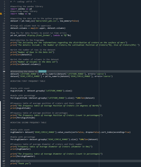
The Result of the above program is below;

The Result clarifies the following;
The major portion of the craters are concentrated near the Equatorial region.
More than 90% of the craters have diameters of about 5Kms.
Number of craters near the Polar region is the least.
Since there were no uncategorised craters in the Data set,Hence there is no missing data.
0 notes